Concepts and math behind 1D and 2D discrete Fourier Transforms for signal and image analysis. Overview of mathematical steps, post-processing, assumptions, and reading of phase and magnitude plots.
Table of Contents
1 INTRODUCTION
In the 1800s, Joseph Fourier showed that periodic functions could be written as an infinite sum of sinusoids. His theory paved the way for Fourier Analysis, a useful tool for signal and data processing.
A 1D signal can be represented as a weighted sum of sinusoids. Image Source: An Interactive Guide To The Fourier Transform, a good explanation by BetterExplained.
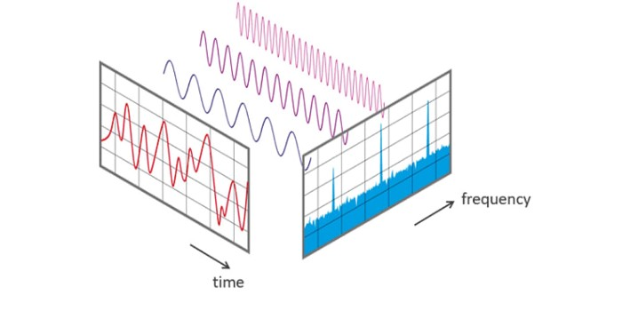
The Fourier Transform is a projection that transforms functions depending on space or time into functions depending on spatial or temporal frequency. Representing functions in the frequency domain allows us to visualize and analyze patterns in the function. The Inverse Fourier Transform allows us to project the frequency function back into the space or time domain without any information loss.
The 2D Fourier Transform has applications in image analysis, filtering, reconstruction, and compression.
2 1D FOURIER TRANSFORM
To understand the two-dimensional Fourier Transform we will use for image processing, first we have to understand its foundations: the one dimensional discrete Fourier Transform.
Understanding the 1D Math
The Discrete Fourier Transform (DFT) turns a 1D array of $N$ discrete, evenly spaced time points, $x$ into a set of coefficients $X$ that describe the weight placed onto $N$ frequency components:
$$X_k = \sum_{n=0}^{N-1} x_n * e^{-i2\pi kn/N}$$
- $n$ specifies the index of the current time point, goes from $0$ to $N-1$
- $k$ is a discrete set of $N$ frequencies, goes from $0$ Hertz up to $N-1$ Hertz
The Inverse Fourier Transform allows us to project the frequency component weights $X$ back into the space or time domain as $x$ without any information loss. It uses a normalization factor of $\frac{1}{N}$ to make the matrix unitary. This lets the inverse FFT formula use the conjugate transpose instead of calculating a matrix inversion (this is faster).
$$x_k = \frac{1}{N} \sum_{n=0}^{N-1} X_k * e^{-i2\pi kn/N}$$
The complex exponential can be decomposed into sines and cosines using Euler’s formula.
$$e^{ix} = \cos(x) + i \sin(x)$$
To understand these equations as a projection, we can rewrite the Fourier Transform and its inverse equation to be in the form of:
$$X = Wx$$ $$x = XW^{-1}$$
The DFT-matrix (W)
The basis matrix $W$ depends on the values of $k$, number of frequency components and $n$, number of time points. Both $k$ and $n$ are vectors with length $N$ that increase from $0$ to $N-1$ by $1$. In the original equations, we sum over all combinations k and n in $e^{i2\pi kn/N}$, so the DFT matrix W is a N-by-N square matrix of elements raised to all combinations of exponents k and n.
Each element of $W$ is a primitive Nth root of unity. For any exponent $kn$, the Nth roots of unity repeat themselves with a period of $N$, as in $w^{kn} = w^{kn \mod N}$. This leads to several patterns of symmetry in W. For example, Eight-point DFT Matrix looks like this:
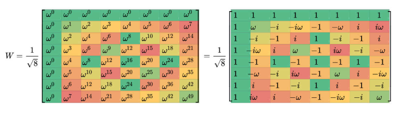
The first image shows w raised to all combinations of k*n. The second image shows the Nth roots of unity repeating themselves with a period of N. The 8 possible values of w are each given a unique color.
We can visualize the DFT Matrix W by graphing the repetition pattern of each row. This representation allows us to see that W is an evenly spaced set of sinusoidal frequencies. The DFT transform is the result of projecting original signal x onto a set of sinusoidal frequencies.
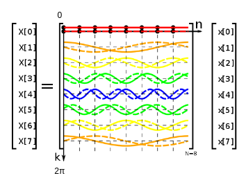
DFT as a matrix multiplication. Real part (cosine) shown by a solid line, and the imaginary part (sine) by a dashed line. From DFT matrix – Wikipedia
Post Projection Processing
Once we have the DFT coefficients $X$, we have to do some post-processing in order to get understandable information.
First, to make the frequency plots easier to read, we shift the frequency components in $X$ so that the zero frequency is in the center and higher frequencies are at the edges.
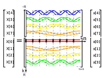
To center a 1D DFT, swap the left and right halves of X.
Next we convert the DFT coefficients $X$ from complex form (real and imaginary parts) into the polar form so we can analyze the magnitude and phase for each frequency.
$$a + ib = r\cos(\theta) + ir\sin(\theta)$$
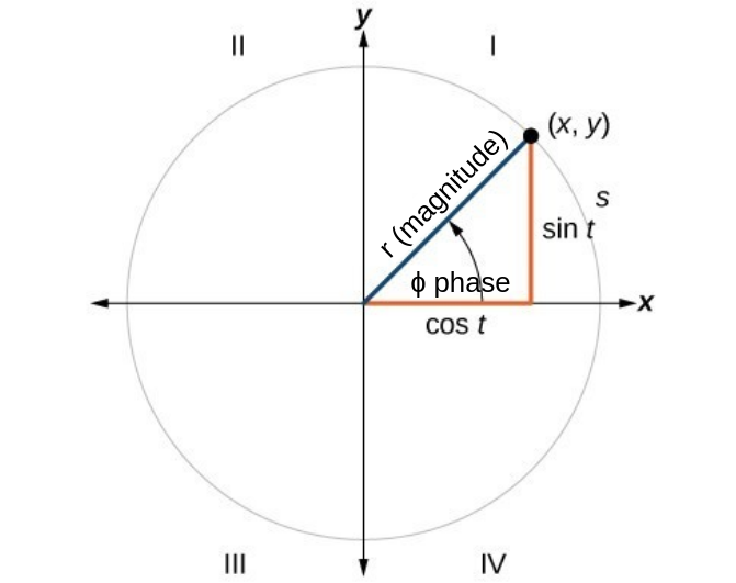
Relationship between complex form and polar form
The magnitude ($r$) tells the amplitude for each associated frequency component.
$$r = \sqrt{a^2 + b^2}$$
The phase ($\theta$) tells the offset of the frequency relative to the start of the time-domain signal.
$$\theta = \arctan(b/a)$$
Once we have the magnitude and phase, we can plot them to see how they change over the different frequency components. The x-axis has the frequency component, and the y-axis has the DFT-coefficient magnitude or phase, depending on the plot.
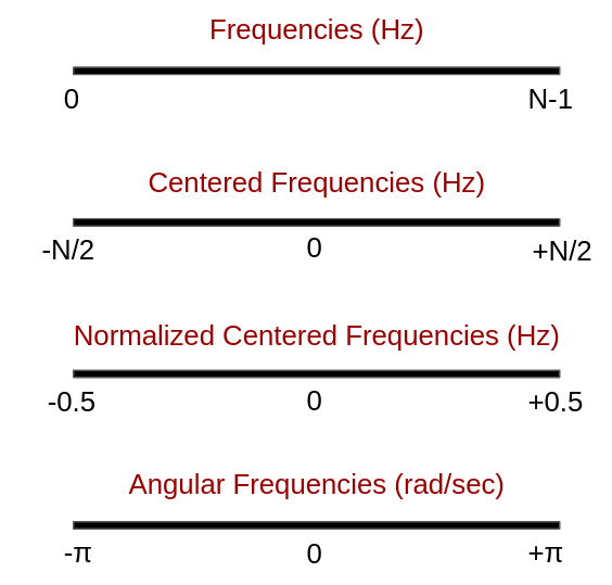
Different but equivalent units for the frequency components on the x-axis
Based on the needed interpretation, the frequency component labels on the x-axis can be in index (0 to N-1), frequencies (Hz), or angular frequencies (radians per second). Frequency can be converted to angular frequency by multiplying by a constant $2\pi$.
Read the 1D Frequency Plots
Let us compare the plots of some simple discrete signals! Here are the magnitude and phase of the DFT coefficients found from projecting a sine wave of 8 Hz, a sine wave of 16 Hz, and a cosine wave of 8 Hz onto a 128-point DFT matrix. Each wave was sampled 128 times over a time-span of 1 second.
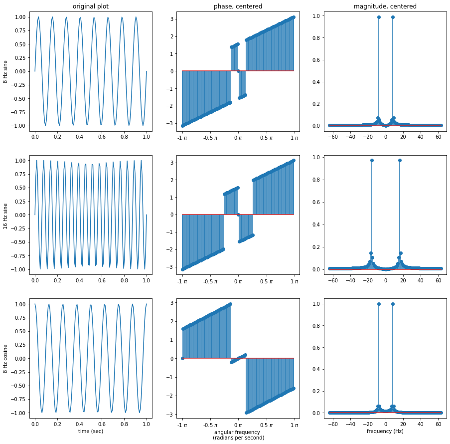
Centered phase and magnitude plots for a sine wave of 8 Hz, a sine wave of 16 Hz, and a sine wave of 8 Hz with a phase offset of π/2 (cosine wave).
The dominant frequencies can be identified from the magnitude plots. In the above plots, the 8 Hz sine wave has magnitude peaks at -8 Hz and +8 Hz, and the 16 Hz sine wave has magnitude peaks at -16 Hz and +16 Hz. The 8 Hz cosine wave has the same magnitude peaks as the 8 Hz sine wave, but its phase plot looks different, indicating the location of the signal components are different. Since half the magnitude plot is a mirror image, the same magnitude information is retained by cropping the x-axis from 0 to 63.
Phase tends to be noisy due to its very small values range ($-\pi/2$ to $\pi/2$) compared to the errors that show up due to rounding calculations in the division operation in inverse tangent (error range of 3 to -3 in this example). In the above phase plots for simple sine and cosine waves, there should only be one dominant frequency, but noise obscures the details.
If we isolate the true dominant frequency components in the phase plot, we get cleaner phase values. At the 8 Hz frequency component, the 8 Hz sine wave has a phase of $\pi/2 = 1.57$ and the cosine has a phase close to zero.
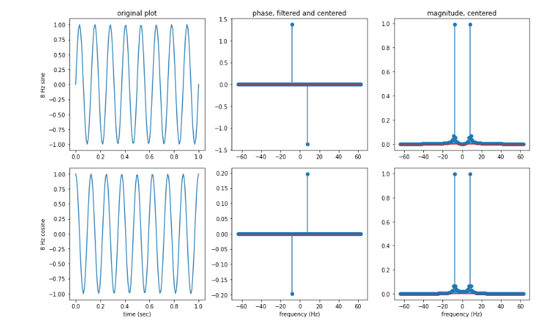
Isolated phase values for 8 Hz frequency component.
3 GENERALIZING TO 2D FOURIER TRANSFORM
Images can be represented as 2D functions $f(x, y)$ varying in spatial coordinates $(x, y)$ in the image plane. Like a 1D wave, every 2D image signal can be decomposed into a series of sine terms.
To visualize the sinuous nature of image signals, we can plot the pixel intensities of the image in a surface plot and observe the top view of its contours. In this view, areas of sharp change, like edges, appear as narrow peaks, and swatches of uniform values, like the evenly colored sky, appear flat with no or low gradual peaks. These patterns have direct parallels with the sharp narrow peaks of high frequency waves and low gradual peaks of low frequency waves.
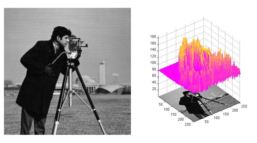
The camera man, a famous image in image processing literature, and his corresponding image surface / Bed Sheet View. From matlab meshCanopy
To represent the 2D image as a sum of 2D sinusoids, we can think of the surface plot from a “Bed Sheet View” perspective (developed by Dr. Steven Brunton at the University of Washington, source: source: Fourier transforms and bed sheet view of images).
The name suggests that an image can be represented by a series of overlaid bedsheets. If we had an infinite number of bedsheets, held each one by its four corners, and oscillated it at one of the Fourier frequencies with the correct corresponding magnitude and phase, then the superposition of all the bedsheets would have creases that looked like the surface plot of an image!
Understand the 2D Math
The 2D discrete Fourier transform projects the NxN image signal $f$ onto a basis of 2D sine and cosine functions (think bedsheets) in order to get the NxN matrix of Fourier coefficients $F$.
The 2D basis functions are matrices ordered by increasing frequency so that the first basis, corresponding to the top left corner of the coefficient matrix, $F(0, 0)$, represents the DC-offset of the image, or average brightness, and the last basis, corresponding to the bottom right corner of the coefficient matrix, $F(N-1, N-1)$ represents the highest frequency. For a square image of size NxN, the two dimensional discrete Fourier transform is given by:
$$F(k, l) = \sum_{i=0}^{N-1} \sum_{j=0}^{N-1} f(i, j) * e^{-i2\pi (\frac{ki}{N} + \frac{lj}{N})}$$
where
- $f(i, j)$ is the value of the pixel at row $i$ and column $j$
- $F(k, l)$ is the Fourier coefficient for each point $(k, l)$ in the Fourier space
- $N$ is the total number of pixels along the x and y direction
The Fourier image can be re-transformed to the spatial domain using the inverse Fourier transform. It uses a normalization factor of $\frac{1}{N^{2}}$ to make the matrix unitary:
$$f(i, j) = \frac{1}{N^{2}} \sum_{k=0}^{N-1} \sum_{l=0}^{N-1} F(k, l) * e^{i2\pi (\frac{ki}{N} + \frac{lj}{N})}$$
In practice, the number of calculations in the 2D Fourier Transform formulas are reduced by rewriting it as a 1D FFT in the x-direction followed by a 1D FFT in the-y direction.
- Mike X Cohen” has a nice animated explanation: “How the 2D FFT works” YouTube
- see NYU online lecture slides 48-49 for details of computational savings
Using the Fast Fourier Transform method computes the 1D DFTs in $\log{2N}$ time. To support this fast, recursive. Some forms of the FFT restrict the size of the input image, often to $N = 2n$ where $n$ is an integer.
Read the 2D Plots
The Fourier Transform math works by assuming the given spatial image is one period in an infinitely repeating spectrum. For example when it looks at the camera man image, it sees:
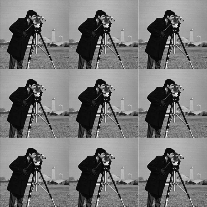
Repeating spectrum of the cameraman image
Like the 1D Fourier Transform, its 2D counterpart also produces a complex output. We can turn the complex output into polar form to observe its magnitude and phase and plot the results.
Like the 1D plots, the magnitude plot is symmetrical. For readability, we can shift the frequencies so the lowest frequency components are in the center and highest frequency components are at the outer edges (swap first and third quadrants, swap second and fourth quadrants).
As in the 1D plots, the phase plot is noisy. Dominant frequencies can be identified from the magnitude plots.
When looking at the magnitude plots, we see a single bright dot (top left corner on magnitude plot, center on shifted magnitude plot). This point corresponds to the DC offset, or average value, of the image and it has a much greater magnitude than the other frequencies.
In order to see more information in the plots, use a log transform to non-linearly scale the magnitude values so the big values are compressed into a smaller range and more information is visible in the plot.
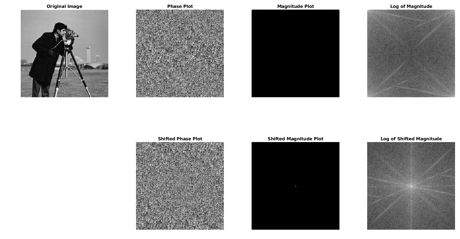
Cameraman FFT magnitude and phase
In the log of magnitude plot, several frequencies are show up. These frequencies describe patterns of repetition like:
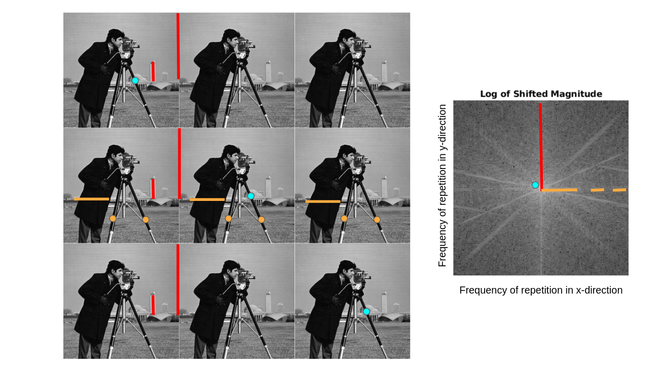
Annotated spectrum of the cameraman image
Bright values closer to the center of the shifted magnitude plot represent a strong pattern of infrequent repetition (no pattern of repetition in the image). Further from the center, bright values indicate strong patterns of more frequent repetition (a pattern of repetition within the image). The sharp diagonals extending outwards into the high frequency components indicate the patterns of diagonals within the image, most likely caused by the tripod legs and tilt of the camera man figure.
For example, the sky and ground create horizontal stripes in the infinite spectrum. Horizontal stripes can be represented by a horizontal 2D sine wave. The horizontal stripes’ FFT magnitude plot has a pattern of vertical dots, indicating the periodic pattern across the y-direction.
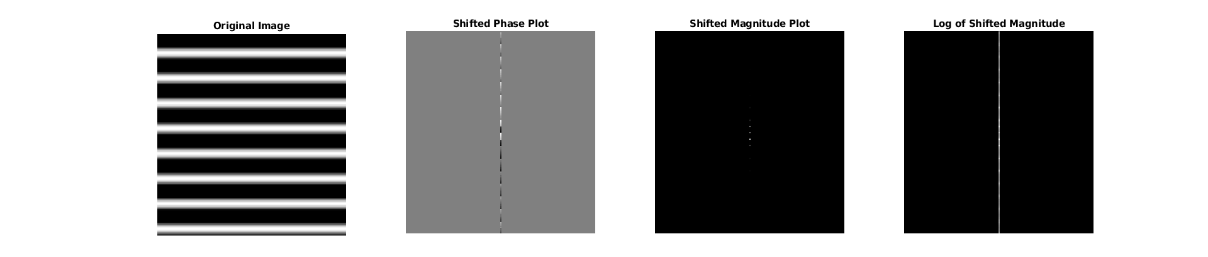
Horizontal sine wave stripes FFT magnitude plot has a pattern of vertical dots indicating the presences of a periodic pattern across the y-direction.
The horizontal stripes’ shifted magnitude plot has three dots, the DC-offset in the center, and two points along the vertical axis. The two points correspond to the dominant frequencies of the image. Similar to reading the 1D shifted magnitude plots, in the 2D shifted magnitude plots we can find the dominant frequencies by calculating the distance from the brightest points to the center of the plot, then converting units from pixel location to basis component frequency indexes.
The log transform compresses the range of the magnitudes and brings more information into the visible range. When analyzing the sine plot, the log of shifted magnitude plot shows all the lesser frequencies that are harmonic multiples of the original frequency.
Exercises
To get a feel for reading patterns from a 2D FFT centered magnitude plot, look at these examples. For each image, think about the repeating unit and directions of periodic repetition. Look back to the annotated cameraman and log magnitude plot image for an example. Remember, low frequency components are in the center of the plot and high frequency components are on the outer edges.
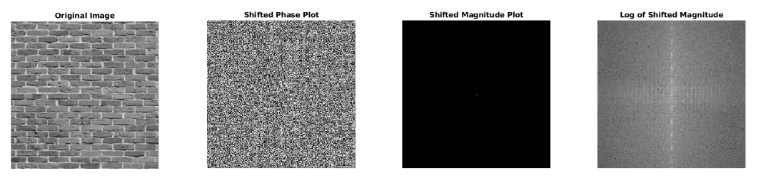
The brick wall image has a stripe pattern in its magnitude plot.
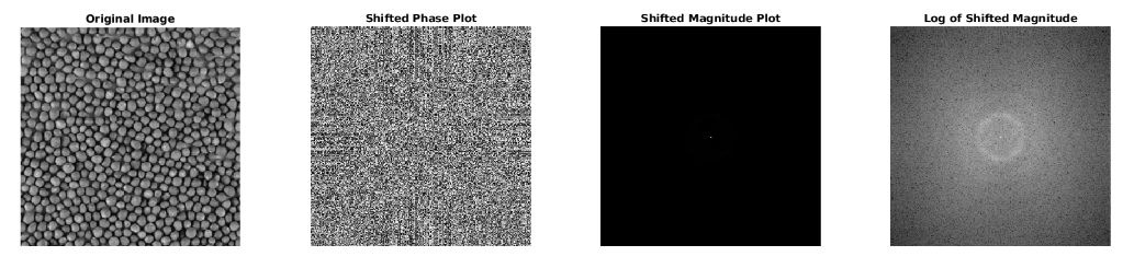
The mustard seed image has circular rings in its magnitude plot.
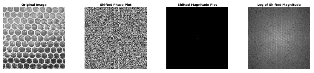
The honeycomb has a hexagonal pattern in its magnitude plot.
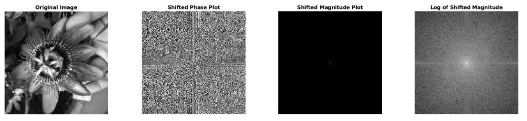
The flower is a more complex image. It’s magnitude plot shows a clear circular pattern of repetition, probably from the patterns of symmetry in the flower, and also vertical and horizontal lines, caused by patterns in the background when the image is represented as an infinite spectrum.
4 FURTHER READING
The Fundamentals of FFT-Based Signal Analysis and Measurement by National Instruments does a nice job explaining basic signal analysis computations, and goes into detail about windowing and the different properties of different windowing functions.
These sites have nice examples and explanations for reading 2D magnitude plots, identifying and removing sources of artificial patterns, and filtering in the frequency domain:
- Image Transforms - Fourier Transform by Hypermedia Image Processing Reference (HIPR2)
- Introduction to the Fourier Transform by John M. Brayer, University of Mexico
- Spatial Frequency Domain by the University of Auckland, New Zealand
Using FFT in Python:
- Fourier Transforms (scipy.fft) — SciPy v1.6.3 Reference Guide is Scipy’s overview for using its FFT library.
- General examples — skimage v0.18.0 docs is a gallery of examples for Scikit-Image Python image processing library. It provides helpful tutorials for thresholding, windowing, filtering, etc.