My team built a servo-driven pan-tilt mount for an infrared proximity sensor. To demonstrate the functionality of our design, we created a 3D scan of a cardboard letter cut in a Z shape. This project involved (1) designing and 3D-printing a pan-tilt servo and IR sensor, (2) programming an arduino to collect scan data, (3) projecting data from spherical coordinates into Cartesian coordinates in order to isolate a cross-section scan of the letter. I was responsible for the CAD mechanical design and making the 3D data projection and visualization.
Table of Contents
Bill of Materials
$15 GP2Y0A02YK0F Sharp Infrared Proximity Sensor
An infrared proximity sensor is an infrared emitter (LED) paired with an infrared detector (photodiode). The detector measures the intensity of the IR light reflected off of an object in its field of view. The output of the sensor is an analog voltage.
Two $4 Hobby Servo Motors
A hobby servo motor is a DC motor connected to:
- a potentiometer (to measure the shaft angle)
- a hardware proportional-integral-derivative (PID) controller (to perform position control)
- a gear train (to increase torque and decrease speed).
A hobby servo is controlled using a square wave form that is pulsed at a fixed frequency. The time that the waveform signal is set to “on” determines what the position of the shaft should be. An arduino board with “pulse width modulation” (PWM) output pin can control a servo motor’s shaft position.
Arduino board + breadboard + assorted circuitry
The Arduino board programmatically controlled the servo motors and received analog outputs from the infrared sensor. The breadboard organized wires, power-supplies, and circuit components. To stabilize the power supply line, a by-pass capacitor of 10μF was inserted between Vcc and GND of the IR sensor.
CAD Design of Pan-Tilt Mount
In this project, I used OnShape because it was free and I was familiar with it. To collect data in a spherical coordinate system, the two servo motor’s axes of rotation and the front of the infrared sensor needed to be in-line. I used the Part Studio feature to define a sketch describing the common references between the mount components. I also made sure the base part had a tabbed base so it could be stabilized with added weight.
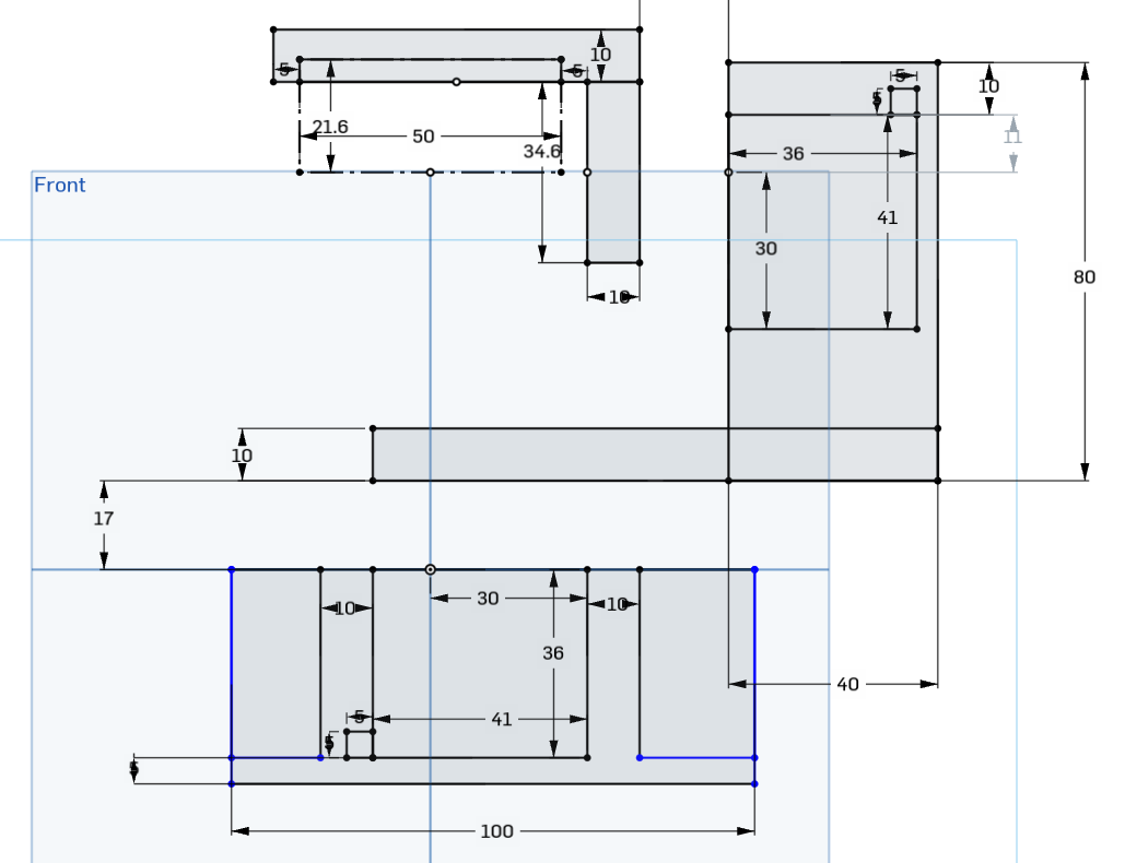
A sketch of the 3 mount components sharing common reference axes.
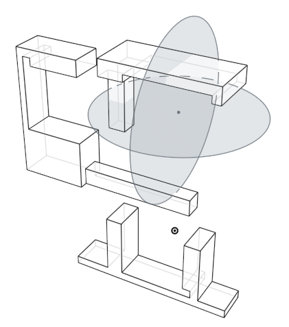
The IR sensor tilts in the y-z plane and pans in the x-y plane.
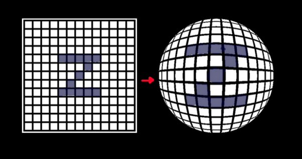
The pan-tilt mechanism’s spherical coordinate system creates a fish-bowl type distortion from the perspective of the IR camera.
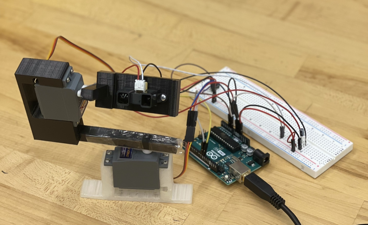
3D printed and assembled mechanism
Scan Demo
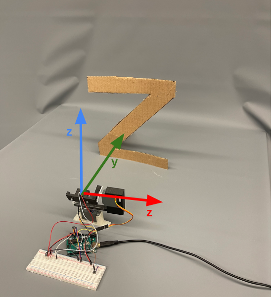
Data collection setup
1. Set-Up and Collection
Orientation: The scanner’s z-axis was pointed upwards, and the scanner’s y-axis was pointed towards the scan object.
Position: The scanner was set up so that when the IR sensor was level, it was pointed at the center of the object. The scanner was 30 cm away from the letter, 60 cm away from the wall.
Code: The arduino board controlled the servos to perform the 2D scan sweep with two nested for-loops. The outer loop drove the tilt servo from 40 degrees to 140 degrees. The inner loop drove the pan servo from 50 degrees to -50 degrees.
## for creating a responsive plot in jupyter notebook
%matplotlib notebook

import math
import pandas as pd
import numpy as np

## importing visualization libraries
import matplotlib.pyplot as plt
import seaborn as sns
from mpl_toolkits.mplot3d import Axes3D

## read spherical scan data from file (data can also be read in real-time over a serial connection)
df = pd.read_csv("serial_output_Z_scan_2D.txt", header=0, names=["ir_read", "orig_tilt_deg", "orig_pan_deg"])
## delete last row with end signal 0,0,0
df = df[:-1]
2. Sensor Output to Distances Calibration
The IR sensor sends out a beam of infrared light, catches the reflected light, and outputs an analog voltage. The relationship between output voltage and distance fits a power law. To reduce noise, multiple sensor reads were taken from each point and averaged.
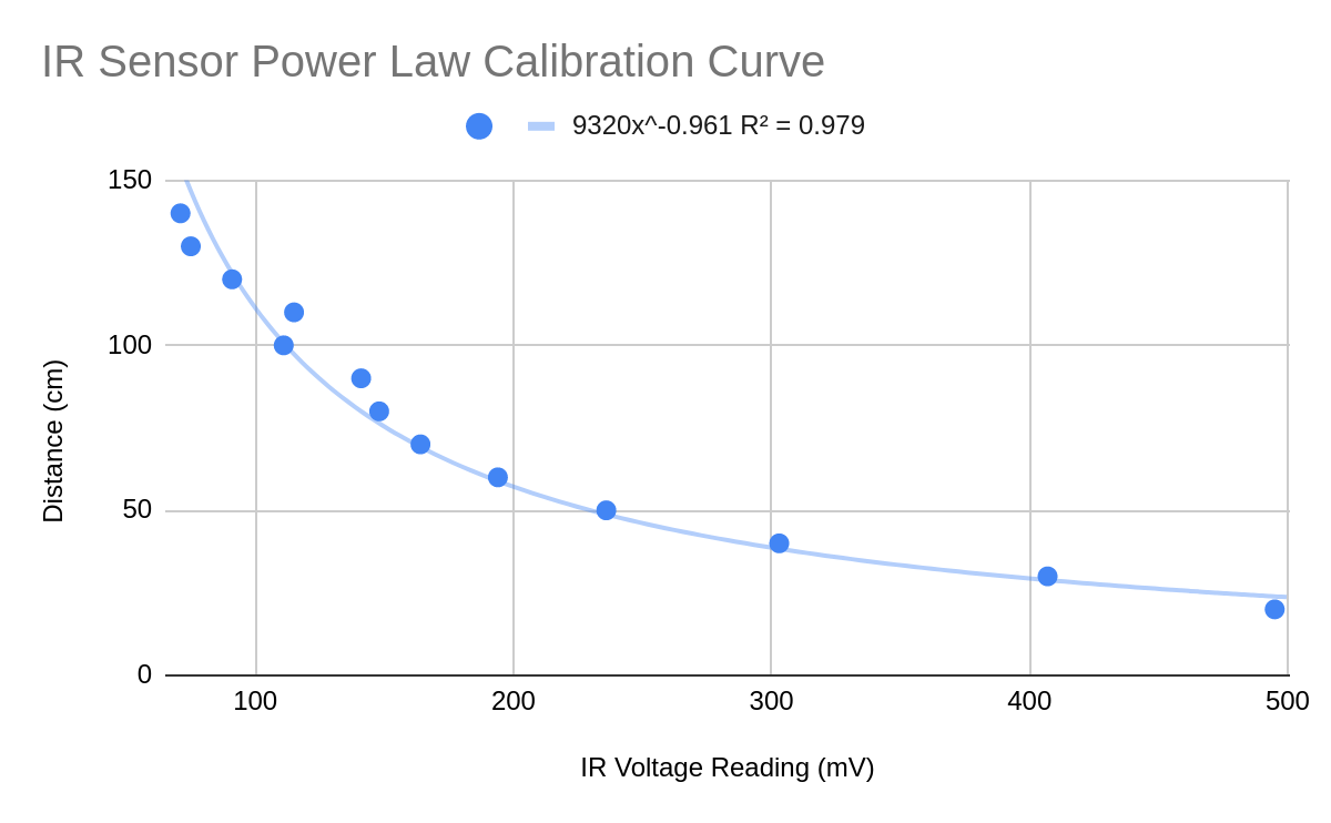
Plot of actual distances vs. infrared sensor output voltage readings
## convert sensor measurement (x) to distance (d)
## y = Cx^-1 (Power Law)
df["distance"] = df.apply(lambda row: 10964 * (1/row["ir_read"]), axis=1)
To test the validity of the curve, we took a series of test points and compared their real distance to the distances predicted by the fitted power-curve equation.
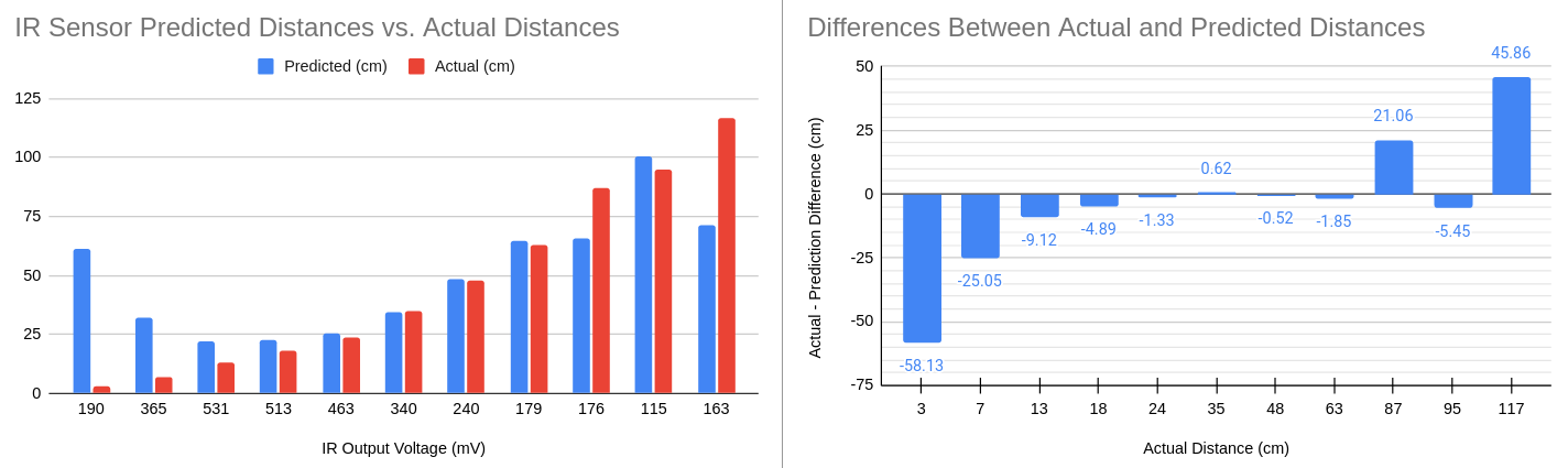
(left) plot of test comparing actual and predicted distances for test infrared sensor output voltage readings; (right) differences between pairs of actual and predicted distances.
According to the spec sheet, the scanner is rated for the 20 to 150 cm range. The has lowest noise and distortion error occurs the 30cm - 60cm range.
3. Accounting for Servo Motor Offsets
The 0-180 pwm input to the servo motors does not line up perfectly with the degrees on the global axes. The servo zero position is offset slightly, by 20 degrees in the tilt servo, and by -60 degrees in the pan servo. This offset needs to be removed before the tilt and pan angles are used in downstream processing.
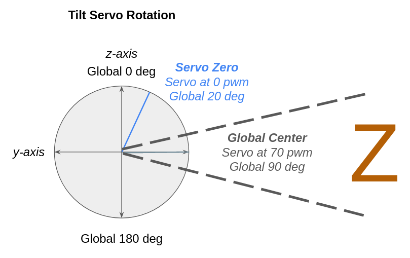
The tilt servo is offset by 20 degrees, so it is centered at 90 - 20 = 70 pwm.
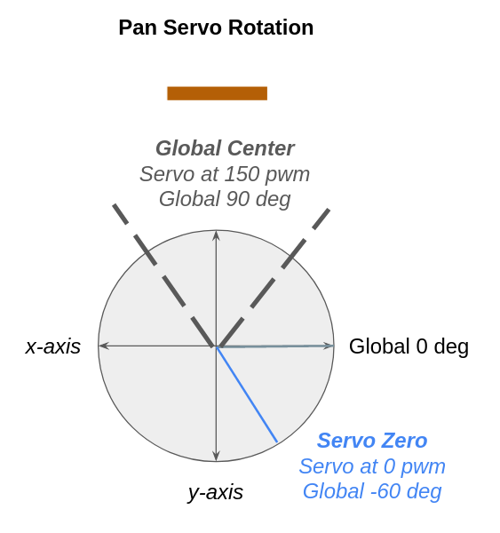
The pan servo is offset by -60 pwm, so it is centered at 90 + 60 = 150 pwm
## account for servo motor offsets
TILT_DEG_OFFSET = 20
PAN_DEG_OFFSET = -60
df["tilt_deg"] = df.apply(lambda row: row["orig_tilt_deg"] + TILT_DEG_OFFSET, axis=1)
df["pan_deg"] = df.apply(lambda row: row["orig_pan_deg"] + PAN_DEG_OFFSET, axis=1)
4. Projection from Spherical to Cartesian Coordinates
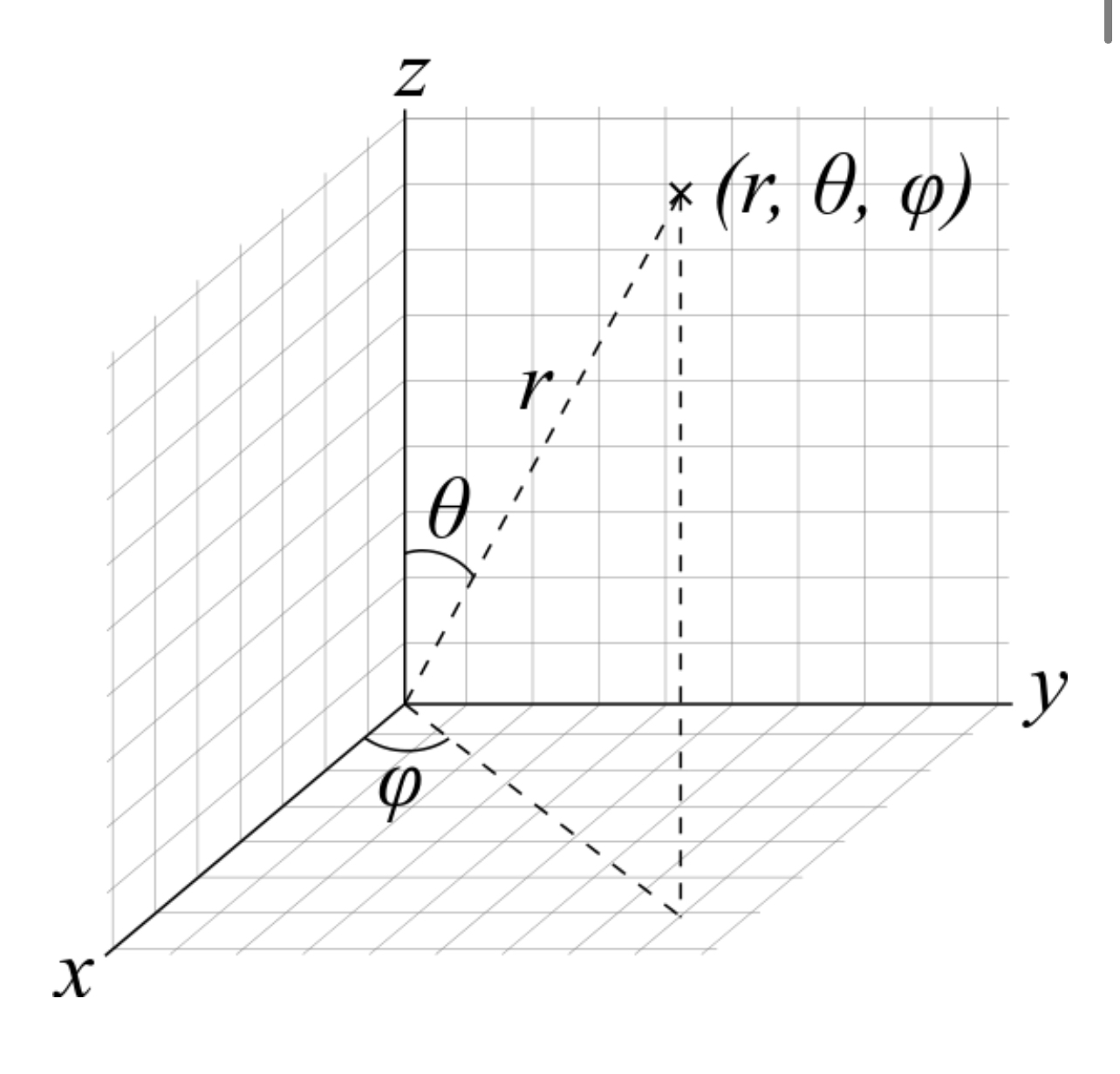
Conversion from Spherical Coordinate Plane to Cartesian Coordinate Plane (Source: LiDAR Basics: The Coordinate System)
The tilt angle is from the Cartesian z-axis to Cartesian y-axis ($\theta$). The pan angle is from the Cartesian x-axis to the Cartesian y-axis ($\varphi$).
In accordance with these relationships, the projection from spherical coordinate system to a 3D Cartesian coordinate system is done with the following equations:
$$x = r \sin(\theta) sin(\varphi)$$ $$y = r \sin(\theta) cos(\varphi)$$ $$z = r \cos(\theta)$$
## convert from degrees to radians
df["tilt_rad"] = df.apply(lambda row: math.radians(row["tilt_deg"]), axis=1)
df["pan_rad"] = df.apply(lambda row: math.radians(row["pan_deg"]), axis=1)

## convert spherical coordinates to Cartesian coordinates
df["xs"] = df.apply(lambda row: row["distance"] * math.sin(row["tilt_rad"]) * math.sin(row["pan_rad"]), axis=1)
df["ys"] = df.apply(lambda row: row["distance"] * math.sin(row["tilt_rad"]) * math.cos(row["pan_rad"]), axis=1)
df["zs"] = df.apply(lambda row: row["distance"] * math.cos(row["tilt_rad"]), axis=1)

## flip axis (because original read was from right-to-left)
df["xs"] = df.apply(lambda row: row["xs"] * -1, axis=1)
5. 3D Scan Visualization
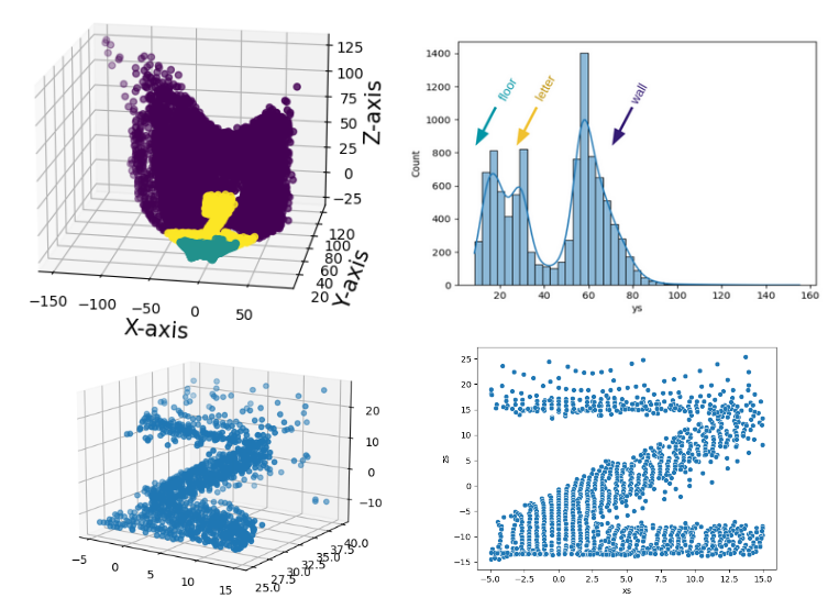
(top) all 3D scan points, annotated by location on y-axis. (bottom) cross section of region containing letter (Z)
To isolate the letter from the wall and the floor, we can look at the point distributions along the y-axis (axis of distance between servo and scanned object).
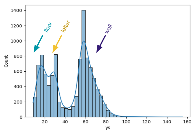
Distribution of scan y-coordinates
We see three main sections:
- 0-30-ish is the floor
- 30-ish is the letter
- 60cm-ish and onwards is the wall
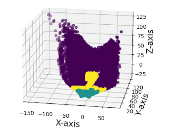
All 3D scan points, positioned in x-z plan labeled according to position along y-axis
Plotting points in the letter location (range y: 25cm-40cm, x:-5cm-15cm) gives this cross-section visual:
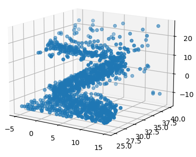
3D scan points in letter location (y: 25cm-40cm, x:-5cm-15cm)
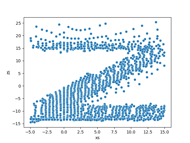
Scan of letter (Z) clearly visible in x-z plane (range y: 25cm-40cm, x:-5cm-15cm)