I have used multiple variations of Principal Component Analysis (PCA) in my research on microbial community analysis. To explain the core theory and assumptions of PCA to my lab group, I fleshed out an analysis of a toy example (eigenfaces) that I had originally seen in class. This analysis reasons about the assumptions of PCA and the effects of applying it to out-of-distribution data by using PCA to perform facial recognition on a dataset of my classmates’ faces.
I was invited to present this project at Łódź University’s SP2021 [virtual] MathUp conference at Łódź University, Poland. The conference was an incredibly fun opportunity to meet fellow researchers and data scientists!
Table of Contents
1 INTRODUCTION
Through this project, I wanted to learn more about the technique of Principal Component Analysis (PCA), namely how to reason about the result of applying PCA on a dataset, and the effects of testing on out-of-distribution data. I set the project up as a facial recognition problem: after teaching a computer what my classmates and I look like, I want the computer to correctly name a person in a picture it hasn’t seen before.
Dataset
For this task, I used grey-scale images of my classmates. Each image was taken against a neutral gray background, eyes and faces were aligned and cropped to 64x64 pixels using a facial detection algorithm. In total, there were 89 subjects, of each subject 4 neutral images and 4 smiling images were taken. I decided to use the neutral images as train data and the smiling images as out-of-distribution test data.
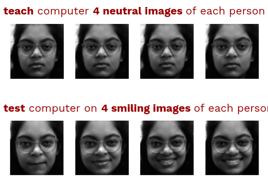
Due to privacy issues and me not wanting to hunt down my classmates for image permission, I am only going to show my face. So here is me!
2 FACIAL RECOGNITION WITH NEAREST NEIGHBOR DISTANCE
To classify a test image, I match it to the closest train image. To find the closest train image, I unroll the image into a vector of pixel values so I am dealing in a vector space where each dimension is the value of one of the pixel features. So I originally had a 64x64 image, now I have a 4096 dimensional vector. This vector representation lets me use the euclidean distance formula to see how close in vector space all the image vectors are. I assume images of the same person are close to each other in vector space.
Graph of distances between a test image, in red, and all the train images. The correct person’s train images are colored blue. Assumption valid: my smiling face is a closer match to my neutral face than to most other training images.
So if I tell my computer to do this pixel by pixel distance comparison for each smiling out-of-distribution test image, it matches with the correct person 93.26% of the time. Which is a decent accuracy considering my train-test distribution discrepancy.
Room for Improvement
The main problem with this approach is bad feature selection. Since each pixel is a feature, we have 4096 features per image, which impacts how we can scale this algorithm. If we have a huge image database or high resolution images, this process gets super slow. Even worse, not only do we have a lot of features, but most of them are either not important or carry redundant information. Our vector space distance formula treats every pixel difference as equally important, but that isn’t how humans look at faces.
In this next part, I will make the computer pick a few important generalized features to look at when deciding the closest match.
Principal Component Analysis (PCA) is an unsupervised machine learning technique that merges correlated variables to transform a big variable set into a smaller, independent, generalized variable set which still contains most of the information.
Sneak preview: correlation matrix of my original dataset with 4096 highly correlated features.
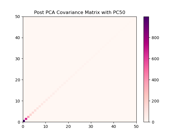
What I want to end up with, a much cleaner correlation matrix of 50 independent features.
PCA Toy Example
So PCA allows us to reduce dimensions with minimal information loss. it does this by picking a better set of features, or axes, to represent our data. In this 2D toy example of not my data, PCA has picked two new axes, principal component 1 and principal component 2. Principal component 1 is in the direction of most variation. Principal component 2 is orthogonal to principal component 1 and it is in the direction of second most variation.
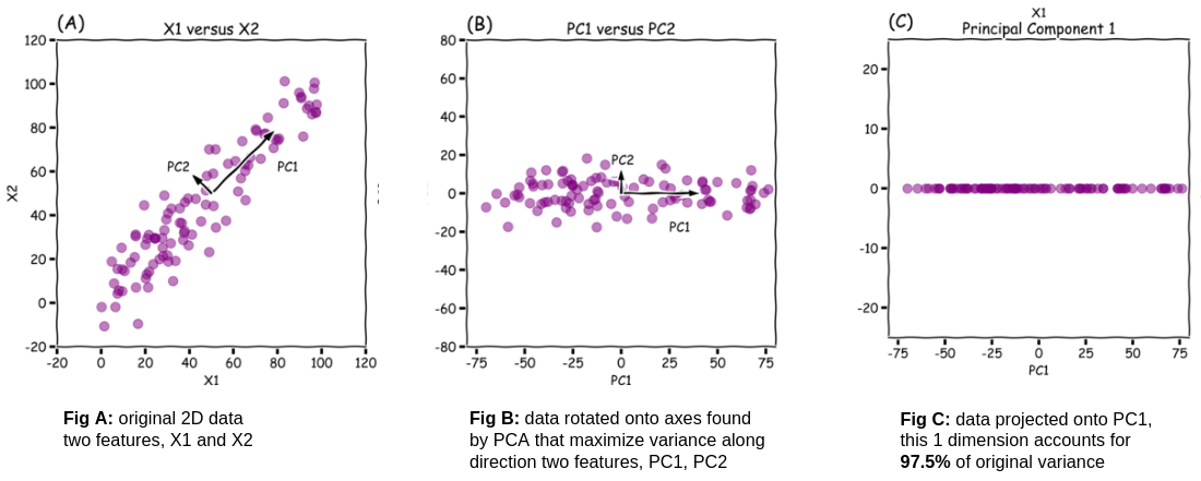
Image Source: Limitations of Applying Dimensionality Reduction using PCA — Roberto Reif
If I rotate my data onto these new axes, all the points still have the same relationship. PC1 holds 97.5% of the variance of the dataset. So if I wanted to drop a dimension, I could get rid of PC2 while only losing 2.5% of the information separating points.
3 FACIAL RECOGNITION WITH PCA NEAREST NEIGHBOR DISTANCE
Step 1. Standardize Dataset
I have to standardize all of my pixel features so they are all on the same scale. This prevents drastic changes (background color) from overshadowing subtle changes (in facial features). I use the standard z-score formula from statistics.
$$standardized\ x_{i} = \frac{x_{i} - mean(x)}{std(x)}$$
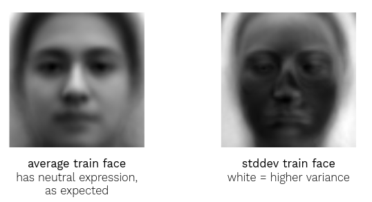
Standardization values for train dataset: average, standard deviation
Standardization allows the algorithm to focus on unusual pixel values, allowing us to encode the assumption that if a pixel varies a lot, drastic changes in it are not important.
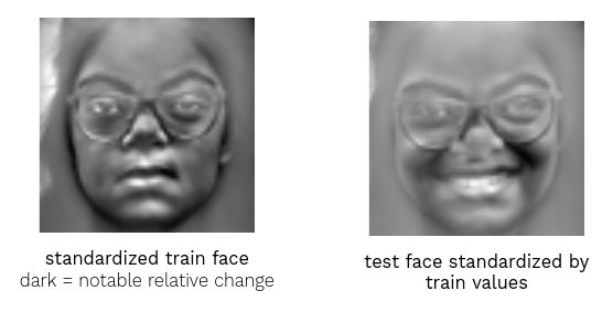
Standardized by train dataset values: train image, test image
Looking at the standardized train face, my black hair has been muted because everything in the background varies a lot and therefore changes in it are less important. My nose and mouth have gotten darker because that area tends to have less change and my pixels in that area are unusually different from the average face so the algorithm pays more attention to those pixels.
My test face has also been standardized by the feature average and standard deviation calculated from the train dataset, which is important because the algorithm shouldn’t know anything about the test data. Because my test face’s features do not follow the train feature distribution, the standardization looks a little washed out.
Step 2. Compute Sample Covariance Matrix from Standardized Train Dataset
My next step is computing the NxN covariance matrix. For each pair of features x, y apply the sample covariance formula.
$$Cov(x, y)= \frac{\Sigma((x_{i} - mean(x))* (y_{i} - mean(y))}{N -1}$$
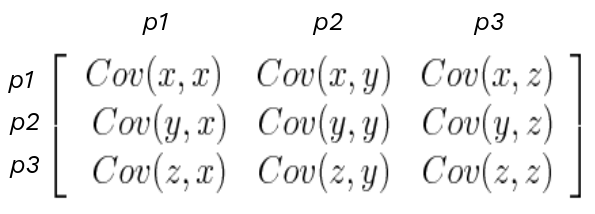
formulation of NxN pixel feature correlation matrix
The covariance matrix lets us identify which features are highly correlated. If features carry the same information, they are redundant and I can replace that set with one feature.
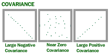
The output of the covariance formula is a number between 1 and -1. A number close to 1 means high positive correlation, a number close to -1 means high negative correlation, and a number close to 0 means the pair of variables are not correlated.
For 64 x 64 pixel images, if each pixel is a feature, there are 4096 features. The train set’s 4096 feature correlation matrix visualized as a heatmap.
The train set correlation matrix has high amounts of yellow and orange, which means it has a lot of highly correlated features. The horizontal and vertical striped pattern means pixels near each other are highly correlated, which we would expect from faces.
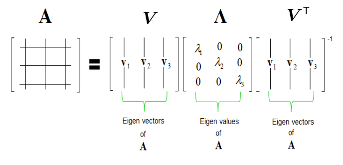
Step 3. Compute Eigenvectors and Eigenvalues of the Covariance Matrix
Eigendecomposition is the heart of PCA. It is smart factoring for matrices. If we give it our covariance matrix, we will get a set of eigenvectors and eigenvalues.
Eigendecomposition via Singular Value Decomposition (SVD). It is like PCA but it works on rectangular matrices as well.
Eigenvectors are orthonormal unit vectors (all perpendicular to each other, have a magnitude of 1). We will use a portion of these as as our new better axes. The eigenvectors are chosen to maximize variance, so the majority of information is explained by the top few eigenvectors.
Eigenvalues, tell us how much variance is explained by each eigenvector direction. We can use the eigenvalues to tell us how much we want to keep the corresponding eigenvector.
Step 4. Pick k Eigenvectors
Since the covariance matrix was a square matrix, the calculated eigenvectors are each 4096 dimensions long. This means I can visualize them like images.
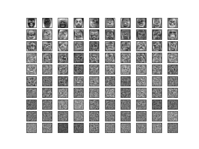
Top 100 training set eigenvectors sorted by eigenvalue. The top eigenvectors capture features varying strongly across all the images. As the eigenvector explains less variance, it captures finer details.
The top few eigenvectors look more like distinct faces (we can call them eigenfaces). Later eigenfaces capture finer details of the faces. Since these were created only from my neutral train set, all the eigenfaces can only explain neutral faces.
So we have 4096 eigenvectors and we only want to keep the top couple. We can estimate how many to keep by looking at variances explained by each eigenvector. Most of these are small since the majority of explained variance is in the top few eigenvectors. We can do a first rough cut by saying if an eigenvalue is less than 1, it explains less variance than an average pixel feature and is not worth keeping.
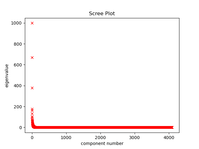
Scree plot of eigenvalues. The last 3,975 eigenvectors have an eigenvalue less than 1.
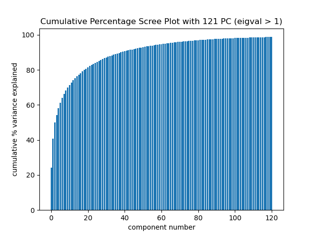
Cumulative percent variance explained plot. Using the top 50 eigenvectors explains 92.7% of the total variance and cumulative percent variance explained levels off after keeping more than 50 components.
So my new feature set is the top 50 eigenvectors of my train dataset.
Step 5. Project and Reconstruct Dataset onto k Eigenvectors
Matrix multiplication can be used to project the images into lower feature space and to reconstruct the projection back into the 4096-feature space to see how much information was lost. The projected train and test images are a weighted sum of the eigenfaces.

To project data onto k PC axes, matrix multiply

To reconstruct and visualize data loss, matrix multiply
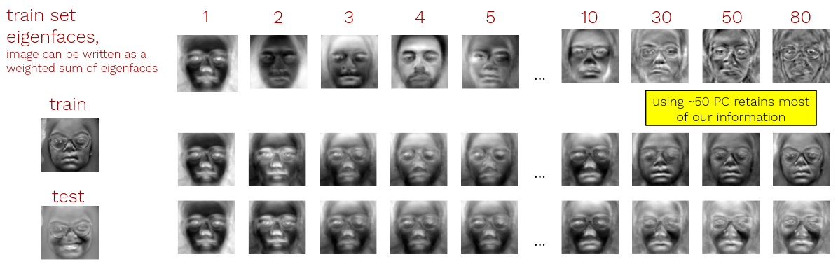
Reconstruction
For the train image, beyond 50 eigenvectors, using more eigenvectors fills in finer details and doesn’t substantially change the image.
For the smiling test image, using more eigenvectors doesn’t allow for a better reconstruction. Data is lost because the axis space (neutral face eigenvectors) cannot fully capture it.
Step 6. Evaluation
Running the distance nearest neighbor algorithm on images projected into only the top two principal component dimensions performs pretty bad. The accuracy of identifying the subject of a smiling test image by label of closest neutral train image is 29.2%. So better than random chance (1.12%) but still pretty bad.
Visualizing the 2D projection lets us understand what is happening:
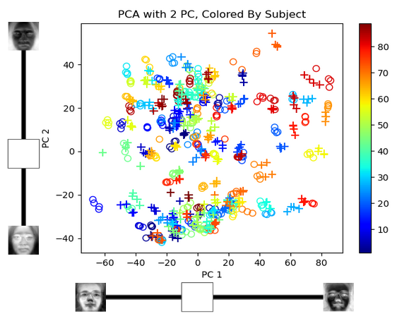
Plot of the weights each image puts on PC1 and PC2. Each person is tagged with a different color, the pluses (+) are smiling images, and the circles (o) are neutral train images.
Amazingly, even when using only two dimensions, train and test images of the same person are grouped closer together. Two dimensions only capture 40.6% of the cumulative variance so it doesn’t separate the people out well (lots of overlap between classes). But if we increase the number of dimensions the separation improves and my closest match finding algorithm becomes much more accurate.
With 50 principal components the closest match classifying algorithm gets an accuracy of 94% on the out-of-distribution data which is better performance AND accuracy than what using the original 4096 pixel dimensions gave.
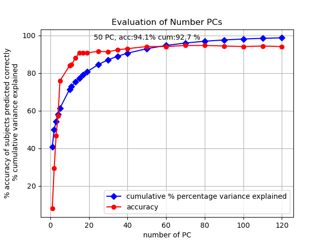
Plot of how accuracy and cumulative percentage variance explained changes as more principal components are used in the projection.
4 APPLICATIONS
Using PCA made all 50 of our dimensions independent, so if we wanted to replace the nearest neighbor distance algorithm with machine learning for classification, it would work much better on our projected dataset (Machine Learning and other pattern searching algorithms perform better on a small number of independent features).
I’ll end by noting PCA is a popular data science algorithm. I’ve seen it used in machine learning, as well as linguistics and microbiology. It is known by many slightly different names and formulas — Principal Coordinate Analysis (PCoA), Singular Value Decomposition (SVD), Latent Semantic Analysis (LSA) — but it’s essentially eigendecomposition.
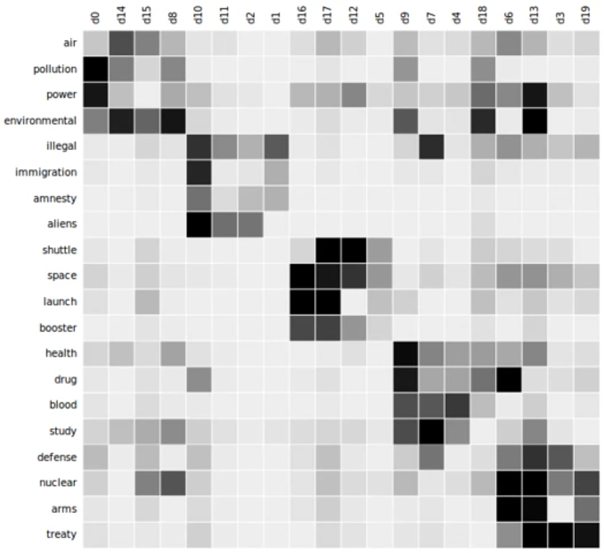
Topic Modeling: merge redundant words instead of pixels (Image Source: Topic model - Wikipedia)
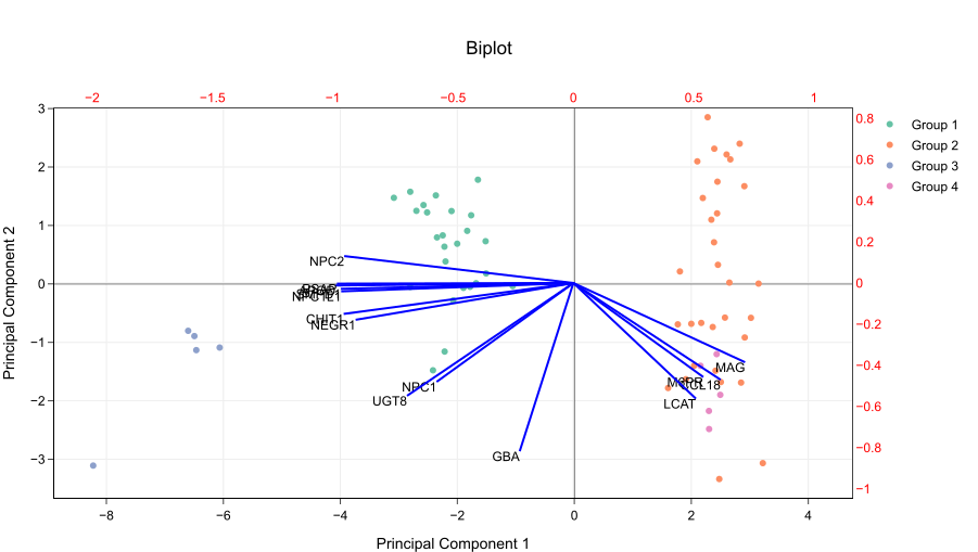
Microbiome Biplot: make PCoA more interpretable by plotting directions in which factors vary. (Image Source: How to read PCA biplots and scree plots)
5 FURTHER READING
- Paper on Eigenfaces for Facial Recognition: M. Turk; A. Pentland (1991). “Face recognition using eigenfaces” (PDF). Proc. IEEE Conference on Computer Vision and Pattern Recognition. pp. 586–591.
- Olin College Eigenfaces Resource: A Face in the Crowd: A Contextualized, Integrated, Intro to Linear Algebra by Olin College Quantitative Engineering Analysis Course
- A Step-by-Step Explanation of Principal Component Analysis
- Eigendecomposition, Eigenvectors and Eigenvalues - Andrew Gurung
- A Complete Guide to Principal Component Analysis — PCA in Machine Learning