Indico Data Solutions provides services to extract information from scanned pdfs. Since their existing OCR + NLP pipeline did not extract handwriting, one of my internship projects involved creating a robust solution to detect and classify handwriting using a deep learning computer vision model.
I started by fine-tuning upon the Faster R-CNN model from the Detectron-v2 framework. Then I tried to improve upon the baseline performance with (i) different pre-training tasks, (ii) multi-label formulation, (iii) strategies to improve small object detection, and (iv) different label sets and datasets. This report documents my methods and finishes with a class confusion analysis and retrospective.
Table of Contents
1 INTRODUCTION
For my internship this summer I was lucky enough to spend my time at Indico Data Solutions as a Research & Development machine learning intern. One of my projects focused on fine-tuning and modifying a pre-trained computer vision object-detection model to detect and classify handwritten marks on documents.
One service Indico provides is extracting information from unstructured documents. This is done by first using OCR to grab printed text from pdfs, and then running a fine-tuned natural language processing model to perform Named Entity Recognition (NER). This existing process does not capture handwritten information that clients might find useful. Utilizing an object-detection model is one way of capturing the missed information.
In this article, I will give an overview of the Faster-R-CNN architecture, discuss experiments and results, and finish by covering future directions to research. For this project, I used the Faster R-CNN model from Detectron-v2 framework, and experimented with (1) different pre-training tasks, (2) multi-label formulation, (3) strategies to improve small object detection, (4) expanded label sets and datasets."
1.1 Datasets
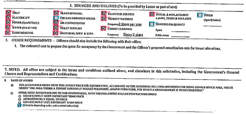
Indico’s labeling team annotated a set of public government lease documents with bounding box locations and multi-labels. Each annotated bounding box could have one or more of the following labels: “Signature”, “Redaction”, “Unfilled Checkbox”, “Filled Checkbox”, “Strikethrough”, “Initials”, “Date”, “Address”, “Name”, “Title”, ”Other Text”, “Stamp”, “Printed”, ”Correction”, “Empty Signature Zone”, “Empty”.
For the baseline experiment, we used a reduced label set (v1) where we kept visually obvious labels with a large number of counts, mapped visually similar labels to the same label, excluded labels with fewer than ~200 counts, and performed aggregate mapping and exclusion.
The original classes “Signature”, “Redaction”, “Unfilled Checkbox”, “Filled Checkbox” were kept, the classes “Initials”, “Date”, “Address”, “Name”, ”Other Text”, were mapped to “Handwriting”, the rare instances of "Stamp", "Empty", "Empty Signature Zone", "Title", "Correction", "Printed", "Strikethrough", “Strikethrough4” were ignored. The multi-label "Handwriting-Signature" was mapped to "Signature", and the multi-labels "Filled Checkbox-Unfilled Checkbox" and "Filled Checkbox-Redaction" were ignored.
All the datasets used in this experiment were public government lease documents.
Lease PNGs Dataset (2339 documents): Used for experiments. Split 80:10:10 (train, test, and dev).
Label Counts in Whole Dataset
all_counts: {‘Signature’: 2333, ‘Other Text’: 1095, ‘Redaction’: 3102, ‘Date’: 1307, ‘Initials’: 3433, ‘Stamp’: 401, ‘Address’: 365, ‘Strikethrough’: 230, ‘Name’: 1024, ‘Filled Checkbox’: 901, ‘Unfilled Checkbox’: 538, ‘Empty Signature Zone’: 65, ‘Printed’: 47, ‘Title’: 65, ‘Correction’: 4, ‘Empty’: 3, ‘Strikethrough4’: 4}
Multi-Label Counts in Whole Dataset
joined_counts: {‘Signature’: 2330, ‘Other Text’: 1041, ‘Redaction’: 3101, ‘Date’: 1093, ‘Initials’: 3403, ‘Initials-Stamp’: 24, ‘Address’: 354, ‘Strikethrough’: 215, ‘Name’: 891, ‘Filled Checkbox’: 898, ‘Unfilled Checkbox’: 532, ‘Date-Stamp’: 202, ‘Empty Signature Zone’: 65, ‘Name-Stamp’: 114, ‘Other Text-Stamp’: 43, ‘Name-Strikethrough’: 2, ‘Name-Other Text-Stamp’: 5, ‘Date-Initials’: 5, ‘Stamp’: 7, ‘Date-Other Text-Signature-Stamp’: 1, ‘Stamp-Strikethrough’: 1, ‘Printed-Title’: 25, ‘Address-Printed’: 9, ‘Name-Printed’: 11, ‘Title’: 38, ‘Correction’: 2, ‘Correction-Other Text’: 2, ‘Stamp-Title’: 2, ‘Address-Empty’: 1, ‘Empty-Initials’: 1, ‘Date-Empty’: 1, ‘Date-Printed’: 2, ‘Signature-Stamp’: 1, ‘Filled Checkbox-Strikethrough’: 1, ‘Strikethrough-Unfilled Checkbox’: 5, ‘Other Text-Strikethrough’: 3, ‘Name-Signature’: 1, ‘Date-Strikethrough’: 3, ‘Address-Stamp’: 1, ‘Filled Checkbox-Redaction’: 1, ‘Filled Checkbox-Unfilled Checkbox’: 1, ‘Strikethrough4’: 4}
FCC PNGs Dataset (2087 documents): Used as an out-of-distribution testing dataset for models trained on the Lease-png dataset.
All Documents Dataset (5871 documents): A bigger, more varied dataset. Used to train final production model. Split 80:10:10 (train, test, and dev).
The full set of documents was comprised of the following data sets:
- Lease PNGs
- FCC PNGs
- TAPAS PNGs
- UCSF batch 1 and 2
- UFO PNGs
1.2 Tough-to-Beat Baseline Model
The Indico object-detection repo supported fine-tuning from the weights of two models:
- baseline-model:
faster_rcnn_X_101_32x8d_FPN_3x_139173657_model_final_68b088 - smaller-baseline-model:
faster_rcnn_R_50_FPN_3x_137849458_model_final_280758
These baseline models have a Faster R-CNN architecture with a backbone net pre-trained on ImageNet classification, and RPN and ROIHead pre-trained on COCO (Common Objects in Context) object-detection tasks
Baseline Results
The object detection evaluation metrics use Intersection-over-Union (IoU) to pair prediction bounding boxes with ground truth bounding boxes.
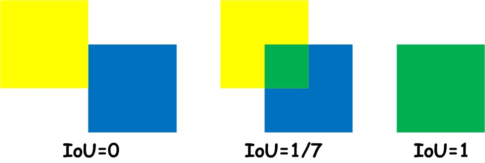
Definition of Object-Detection: Intersection-over-Union (IoU)
The models that assigned a single label to each bounding box were evaluated with COCOEvaluator’s metrics for average precision, average recall, and per class average precision.
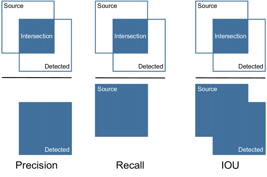
Definition of Object-Detection: Precision, Recall, IoU
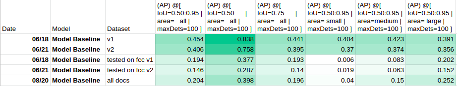
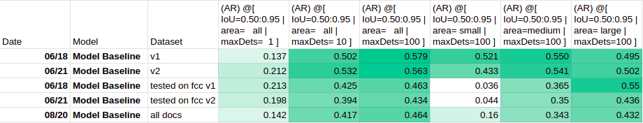
Average Precision (AP) and Average Recall (AR) is measured out of 100 points t various thresholds. AP Numbers in the 40s are good. We care most about AP per class and AP50. For metrics tables in this report, cells are colored linearly with respect to the min and max values of the given table.
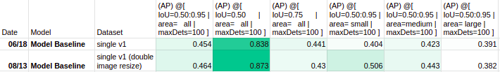
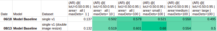
Fine-tuning the baseline and smaller-baseline models to the handwriting detection task using label set v1 and Lease PNG dataset gave the following results:
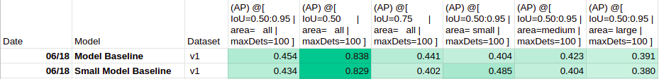
Average Precision (COCOEvaluator)
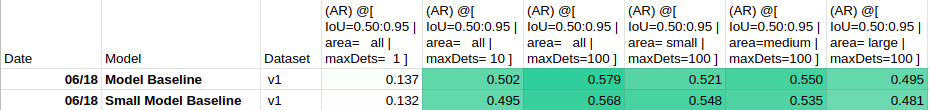
Average Recall (COCOEvaluator)

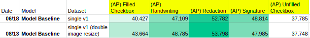
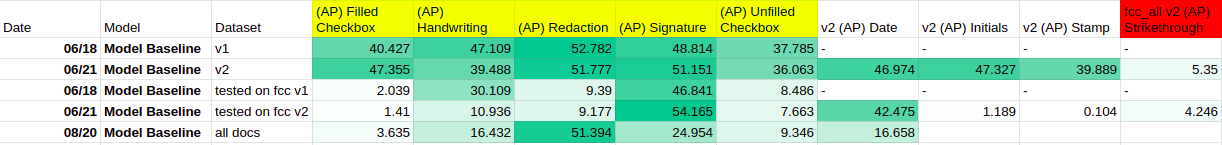
Per Class Average Precision (COCOEvaluator)
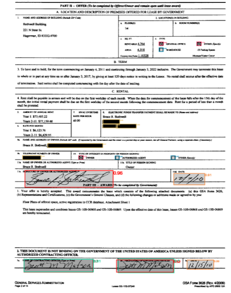
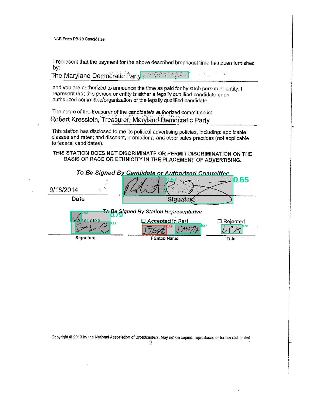
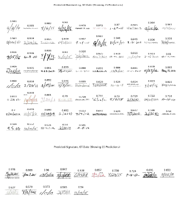
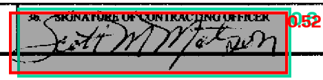
Lease PNG document image (LID07240-Lease-a_Z-1.png) with fine-tuned baseline model predictions.
COLOR KEY
- Predictions have tinted fill, ground truth label has no fill
- pink: Filled Checkbox
- blue: Unfilled Checkbox
- teal: Handwriting
- red: Signature
- yellow: Redaction
- orange: Date (in label set v2 and v5)
The baseline model performs quite well. The following analysis investigate error modes and attempts to beat the baseline model.
2 BACKGROUND INFORMATION
2.1 Overview of Detectron-v2’s Faster R-CNN with FPN
Detectron2 is Facebook AI Research’s library for object detection and segmentation algorithms. In this project, I used the Faster R-CNN with Feature Pyramid Network (FPN) architecture, which is the basic multi-scale bounding box detector with high accuracy in detecting tiny to large objects. It has three main parts: Backbone Network, Region Proposal Network, and ROI Head (Box Head). Becoming familiar with the Detectron-v2 framework and the Faster R-CNN with FPN architecture was a major part of my learning experience this summer. See the Appendix for my notes and observations.
Useful Resources
- Detectron-v2 GitHub Repo
- Papers:
- Useful 5-part explanation of repo structure and Faster R-CNN with FPN implementation By Hiroto Honda
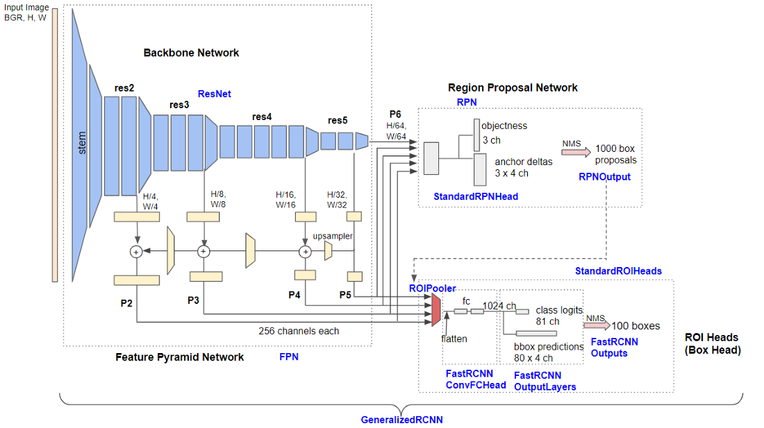
Detailed architecture of Base-RCNN-FPN. Blue labels represent detectron-v2 class names. (Source: Digging into Detectron 2 — part 1 | by Hiroto Honda)
2.2 Overview of Fine-Tuning
Fine-tuning is a technique that lets you take the weights of a trained neural network (source model) and use it as initialization for a new model (target model) that you want to train on data from the same domain. This technique lets you achieve good performance with a faster training time and small dataset size.
Useful Resources - Good conceptual understanding of fine-tuning
When I fine-tune on a detectron-v2 model, I get this warning message:
Skip loading parameter ‘roi_heads.box_predictor.cls_score.weight’ to the model due to incompatible shapes: (81, 1024) in the checkpoint but (5, 1024) in the model! You might want to double check if this is expected.
Skip loading parameter ‘roi_heads.box_predictor.cls_score.bias’ to the model due to incompatible shapes: (81,) in the checkpoint but (5,) in the model! You might want to double check if this is expected.
Skip loading parameter ‘roi_heads.box_predictor.bbox_pred.weight’ to the model due to incompatible shapes: (320, 1024) in the checkpoint but (20, 1024) in the model! You might want to double check if this is expected.
Skip loading parameter ‘roi_heads.box_predictor.bbox_pred.bias’ to the model due to incompatible shapes: (320,) in the checkpoint but (20,) in the model! You might want to double check if this is expected.
These warnings appear because the source model’s final layer had shape and weights to project into 80+1 and 80x4 tensors, but the new target model has a different number of classes and therefore has a different final layer projection.
3 FINE-TUNE ON MODELS PRE-TRAINED ON DOCUMENTS
The first experiment involved fine-tuning on Layout Parser Models.
- Layout Parser Website: https://layout-parser.github.io/
- Layout Parser Repo: https://github.com/Layout-Parser/layout-parser
Despite being pre-trained on “natural” images, the ImageNet + COCO pre-trained baseline models seem to generalize well to document images. But perhaps models pre-trained on documents would do even better. To test this hypothesis, I could fine-tune on layout-parser models that are pre-trained on document images.
Layout Parser offered the following models:
- HJDataset – trained on Japanese documents
- Prima – too small
- PubLayNet – Incompatible large model of type mask rcnn, trained on academic papers
- LayoutParser gives the following note: “For PubLayNet models, we suggest using
mask_rcnn_X_101_32x8d_FPN_3x modelas it’s trained on the whole training set, while others are only trained on the validation set (the size is only around 1/50). You could expect a 15% AP improvement using themask_rcnn_X_101_32x8d_FPN_3xmodel.”
- LayoutParser gives the following note: “For PubLayNet models, we suggest using
- Newspaper Navigator – large but trained on Newspapers
- TableBank – large but trained on academic papers
None of the models were perfect for the domain use-case of unstructured business documents. Of the available options, the largest Faster-RCNN models of NewspaperNavigator and the TableBanks seemed like the best choices. We decided to compare the following bounding box object detection models to the model baseline and small model baseline:
- NewspaperNavigator:
faster_rcnn_R_50_FPN_3x - TableBank:
faster_rcnn_R_50_FPN_3x - TableBank:
faster_rcnn_R_101_FPN_3x
Porting the models into Indico’s platform for fine-tuning was quite simple since both layout-parser repo and indico’s object-detection repo were both built on top of detectron-v2. I just had to download the model weights and configuration file from the layout parser zoo and make a couple minor code changes.
3.1 Check for Porting Discrepancies
I wanted to make sure that the LayoutParser platform and indico object-detection platform returned the same outputs given the same input image and model, and that there were no pre- or post-processing discrepancies.
To check for preprocessing discrepancy, I saved the image right before model prediction and checked that the images were identical.
torch.all(loaded_indico["image"].eq(loaded_layoutparser["image"]))
tensor(True)
Then, to check that predictions matched, I wrote a script to load model weights into indico’s object-detection platform and predict with them directly (without fine-tuning).
path to image: data/fcc_2c3a1ab2-0c2a-4a9e-96d4-1715719c1fde_01.png
Trying out indico…
** _load_base_model cfg.MODEL.WEIGHTS /indicoapi_data/layout_parser_models/TableBank_faster_rcnn_R_50_FPN_3x.pth
INDICO OUTPUT [[{’label’: ‘Table’, ’left’: 126, ‘right’: 1141, ’top’: 716, ‘bottom’: 1120, ‘confidence’: 0.9895569682121277, ‘image’: <_io.BytesIO object at 0x7f569f52e0b0>}]]
Trying out layout parser…
LAYOUT PARSER OUTPUT Layout(_blocks=[TextBlock(block=Rectangle(x_1=126.4218521118164, y_1=716.7941284179688, x_2=1141.1806640625, y_2=1120.6494140625), text=None, id=None, type=Table, parent=None, next=None, score=0.9895569682121277)], page_data={})
3.2 Results
Each model was trained on Lease PNG label set v1 and evaluated on the test split.
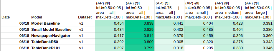
Average Precision (COCOEvaluator)
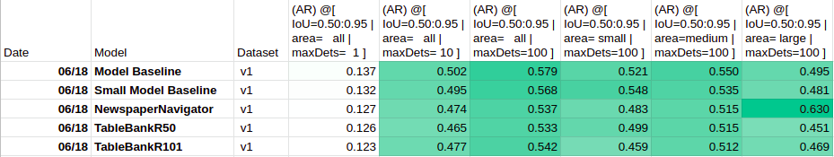
Average Recall (COCOEvaluator)
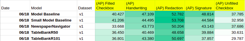
Per Class Average Precision (COCOEvaluator)
In these metrics, the baseline model did slightly better overall, especially in Average Precision by class. It was followed closely by the small model baseline and NewspaperNavigator, with both TableBanks doing the worst. The ported layout-parser models did not realize a significant improvement when detecting the target classes. Their pre-training on detecting newspaper components and detecting tables in academic papers perhaps did not give them an edge in the task of detecting filled and unfilled checkboxes, signatures, redaction, and handwriting.
4 EXPAND THE LABEL SET
Since the baseline model had good evaluation numbers on label set v2, the next step was expanding the label set to handle tougher classes. The new label set (v2) had 9 classes, keeping the 5 classes from v1 and adding 4 new, somewhat visually obvious classes with 200+ counts: “Date”, “Initials”, “Stamp”, and “Strikethrough”.
Since “Stamp” and “Strikethrough” looked like very visually distinguishable classes, any multi-label that included the “Stamp” label and “Strikethrough” label were mapped to the “Stamp” class and “Strikethrough” class, respectively, to make the new label set easier to learn.
The label set v2 Lease-PNG dataset had the following total instance counts:
all_counts: {‘Signature’: 2333, ‘Date’: 1299, ‘Initials’: 3427, ‘Handwriting’: 2496, ‘Redaction’: 3101, ‘Stamp’: 401, ‘Filled Checkbox’: 899, ‘Unfilled Checkbox’: 537, ‘Strikethrough’: 234}
4.1 Results
Note: The performance of the model on v1 and v2 cannot be directly compared because their train and test splits contained different documents. Despite this, some conclusions can still be drawn. Each model was trained on the Lease-PNG dataset and evaluated on the test split.
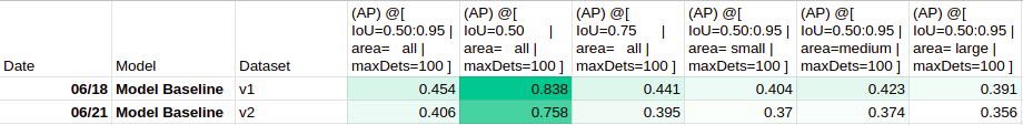
Average Precision (COCOEvaluator)
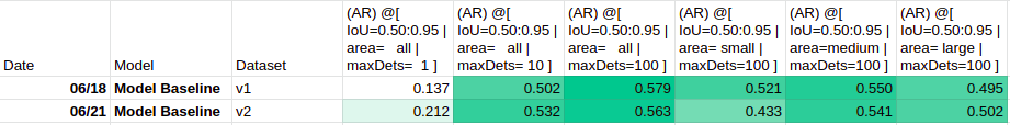
Average Recall (COCOEvaluator)

Per Class Average Precision (COCOEvaluator)
Overall, the model trained on v2 had a decent per class AP on the expanded v2 label set, with the exception of the ‘Strikethrough’ class.
4.2 Analysis of Class Confusion Via Visual Inspection
Additionally, visual inspection of the predictions showed that the model sometimes struggled with distinguishing between ‘Filled Checkbox’ vs. ‘Unfilled Checkbox’ and ‘Stamp’ vs. ‘Date’.
At first, to get a sense of the error modes of the model predictions, I glanced through the visualized model predictions and noted down interesting and common errors. Following further analysis I came to realize that some of my conclusions were subject to confirmation bias (you see an error early on so you look for that error more than other errors). I have kept this analysis here because (1) it was an important realization to learn, and (2) this analysis led us to future decisions. For the more objective analysis I performed later, see the qualitative and quantitative analysis section below.
Strikethrough
Instances of ‘Strikethrough’ had a fair bit of variation (scribble, line through word, line through paragraph). There were a small number of examples to learn from (there were less than 230 instances of ‘Strikethrough’ in the training set), and some examples were not labeled, so the model’s poor performance was understandable.
Filled Checkbox vs. Unfilled Checkbox
In the “Filled Checkbox” vs. “Unfilled Checkbox”, the predictions sometimes missed the checkbox or labeled it incorrectly. There weren’t many errors here:
Lease PNG document image (LCT04791-Lease-0.png) as an example of predictions missing the very small checkboxes at the bottom of the page. The model predicted these correctly on another similar document (LFL61825-Lease_Z-0.png) so maybe the skew on this particular document affected it here.
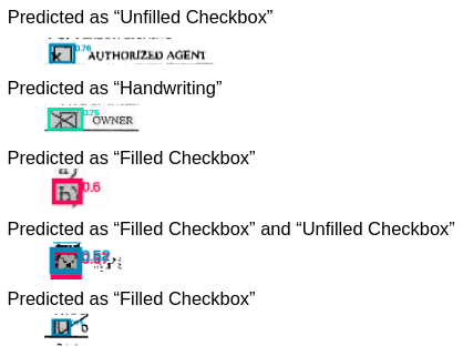
More examples of incorrectly predicted checkboxes identified via visual inspection (aside from these, the checkboxes from the Lease_PNGs dataset were generally neat and marked with an even X).
Stamp vs. Date
The ‘Stamp’ vs. ‘Date’ confusion could be attributed to my label aggregation decision. In label set v2, I had mapped all ground truth [‘Date’, ‘Stamp’] multi-labels to the ‘Stamp’ class, and the model sporadically predicted those as “Date” or “Stamp” (in my Confusion Matrix based analysis I found out that this occurred less frequently that I had first assumed).
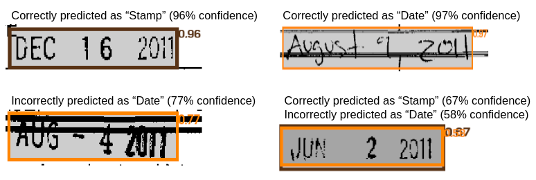
Examples of model predictions of Date (Orange) and Stamp (Brown) from Lease-PNG v2 test split.
Despite the low frequency, the nature of this class confusion still identified a major issue: there is no right way to map two different axes of variation onto one set of single labels without taking the explicit set of all pairs.
In the single label scheme, if a “Date-Stamp” has a mapped ground truth of “Stamp” and it was predicted as “Date” or two separate “Date” and “Stamp” predictions, the Softmax loss function and metrics say that the model is completely wrong.
4.3 Considerations on an Alternative Formulation
Using a pairing as a single label (e.g. “Date-Stamp”) would give the model the option to label a predicted instance as both “Date” and “Stamp”, but there are some problems with this solution. If the ‘Date-Stamp’ pairing was a label, at ~200 counts, the class would have a low instance count. Furthermore, the model would not be able to use its knowledge of the “Date-Stamp” class to improve its prediction on other “Date-” or “Stamp-” hybrid classes. At this point, we decided to experiment with a multi-label model formulation to allow the model to learn multiple axes of variation at once and take better advantage of the original multi-label formulation of the ground truth label set.
There is an alternative formulation that might have been better suited to this problem: using a multi-task concept, where there is one loss for style (e.g. ‘Stamp’) and one loss for content type (e.g. ‘Date’). However, the indico platform currently has a multi-label concept, but not a multi-task concept, so implementing a multi-task formulation for this problem would have been harder to support and less generalized.
5 MULTI-LABEL OBJECT DETECTION
5.1 Detectron-v2 Modifications
Making the model handle multi-label required changing (1) the label representation from scalar class index to list of class indexes, and (2) the classification loss from Softmax to binary cross entropy.
The original single-hot encoding was a tensor of length num_classes+1, where only one position can hold a 1 and the last position indicates the background class. The new multi-hot encoding is a tensor of length num_classes, where any number of positions can hold a 1, and a vector of all 0s indicates the background class.
Here is a list of parts of detectron-v2 had to change to be compatible with the multi-label formulation:
- Create
MultilabelDatasetMapperclass (extendsDatasetMapper)- Change
annotations_to_instancesfunction to handle gt_classes in multi-label format (instead of a list of int classes, handle as a list of multi-hot encodings) CreateMultilabelFastRCNNOutputsclass (extendsnn.Module, same interface as:class:FastRCNNOutputLayers.) - Change
fast_rcnn_inference_single_imageto not remove last column because vector is multi-label and to handle post NMS merging of multiplepred_classesand scores into a list corresponding to Boxes - Change
lossesto cat multi-label class gt and predictions and to usesigmoid_cross_entropyinstead of Softmax classification loss - Change
box_reg_lossto keep instances that are labeled foreground (not zero vectors), and handle getting class-wise box regression loss if multiple classes apply OR (better) inbox_reg_lossuse class-agnostic bounding box regression by settingMODEL.ROI_BOX_HEAD.CLS_AGNOSTIC_BBOX_REGin the model config file. This option modifies the final box projection layer to output a tensor of length 4, instead of a tensor of length num_classes x 4.
- Change
- Create
MultilabelROIHeadsclass (extendsStandardROIHeads)- Change
_init_box_headto useret["box_predictor"] = MultilabelFastRCNNOutputs(cfg, ret["box_head"].output_shape) - Change
_sample_proposalsto handlegt_classesin a multi-label format - Change
subsample_labelsto handle getting indexes of foreground and background when they are in multi-label vector format
- Change
- Comment out lines that complain when multi-label
- The config function for
build_detection_train_loaderandbuild_detection_test_loadercalledget_detection_dataset_dictswhich had lines that complained when instances had a multi-label format
- The config function for
- Evaluation
- Write a
MultilabelEvaluator, which is aCOCOEvaluatormodified to handle a binary evaluation problem. For the given class, it keeps the annotations of that class. - Use a list of
MultilabelEvaluator, one for each class.
- Write a
5.2 New Label Sets
Multi-label set v1: simplest v1 Lease-PNG multi-label set, easily compare its performance to the baseline single-label model.
all_counts: {‘Handwriting’: 6796, ‘Redaction’: 3101, ‘Signature’: 2331, ‘Filled Checkbox’: 899, ‘Unfilled Checkbox’: 537}
Multi-label set v3: the “Checkbox” and “Unfilled Checkbox” had a drop in AP score for the multi-label model compared to the single-label model. Introduced a separate “Checkbox” class to multi-label mark both “Filled Checkbox” and “Unfilled Checkbox" to help the multi-label model detect checkboxes better,
all_counts: {‘Handwriting’: 6796, ‘Redaction’: 3101, ‘Signature’: 2331, ‘Filled’: 899, ‘Checkbox’: 1436, ‘Unfilled’: 537}
Multi-label set v4: removed the redundant “Unfilled Checkbox” class since its attributes overlapped with the “Checkbox” class.
all_counts: {‘Handwriting’: 6796, ‘Signature’: 2331, ‘Checkbox’: 1439, ‘Filled’: 901, ‘Redaction’: 3102}
5.3 Results
Note: The performance of the model on label sets v1, v3, and v4 cannot be directly compared because their train and test splits contained different documents. Despite this, some conclusions can still be drawn. Each model was trained on the Lease-PNG dataset and evaluated on the test split.
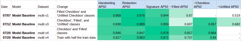
Per Class Average Precision 50 for multi-label models (Modified Binary COCOEvaluator). *For single-label v1 model overall AP50 = 0.838
![Per Class Average Recall for multi-label models (Modified Binary COCOEvalulator) *For single-label v1 model overall (AR) @[ IoU=0.50:0.95 | area= all | maxDets=100 ] = 0.502](/projects/handwriting-detection-with-faster-r-cnn-plus-experiments/img/eval_AR_multi.png)
Per Class Average Recall for multi-label models (Modified Binary COCOEvalulator) *For single-label v1 model overall (AR) @[ IoU=0.50:0.95 | area= all | maxDets=100 ] = 0.502
Per Class Average Precision for single- and multi-label models (Modified Binary COCOEvaluator and COCOEvaluator)
Overall, there was not a significant improvement from switching from single-label to multi-label or from using differently aggregated multi-label sets. The multi-label formulation appears to do 5-10 points worse in Unfilled Checkbox AP.
In both the single and multi-label formulation, the bigger size classes (‘Handwriting’, ‘Signature’, ‘Redaction’) had AP numbers that were 10+ points higher than the smaller size classes (‘Filled Checkbox’ and ‘Unfilled Checkbox’). Looking at multi-label AP50, the model seems decent at identifying a checkbox, and worse at telling whether the checkbox was filled or unfilled.
6 BETTER SMALL OBJECT DETECTION
Detecting small objects is a known trouble spot for object-detection models.
Useful Resources
- Anchor Boxes — The key to quality object detection (best, quick read)
- Tackling the Small Object Problem in Object Detection
- Small objects detection problem | by Quantum
There are two main approaches I decided to examine: (1) increase image resolution so small objects are bigger, and (2) adjust anchor sizes for better small object bounding box regression.
6.1 Visualize Feature Map
In the default DataMapper, the following transform is applied to all the images:
[ResizeShortestEdge(
  short_edge_length=(640, 672, 704, 736, 768, 800),
  max_size=1333,
  sample_style='choice'),
  RandomFlip()
  ]
Images are rescaled to have a shortest edge of length 800 (for test) or randomly chosen from (640, 672, 704, 736, 768, 800) (for train). The RandomFlip means the DataMapper randomly chooses some images to get a horizontal flip transform.
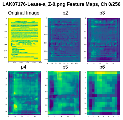
Given LAK07176-Lease-a_Z-0.png as the input image, the FPN + ResNet backbone net creates the following 5 feature maps (visualized channel 0)
If the original image is 2556x3305 pixels, it is rescaled to be 800x1056.
- feature map p2 is created with a stride of 4 (200x264)
- feature map p3 is created with a stride of 8 (100x132)
- feature map p4 is created with a stride of 16 (50x66)
- feature map p5 is created with a stride of 32 (25x33)
- feature map p6 is created with a stride of 64 (12x16)
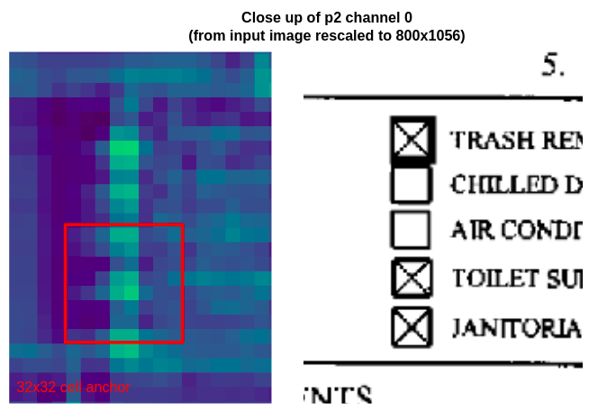
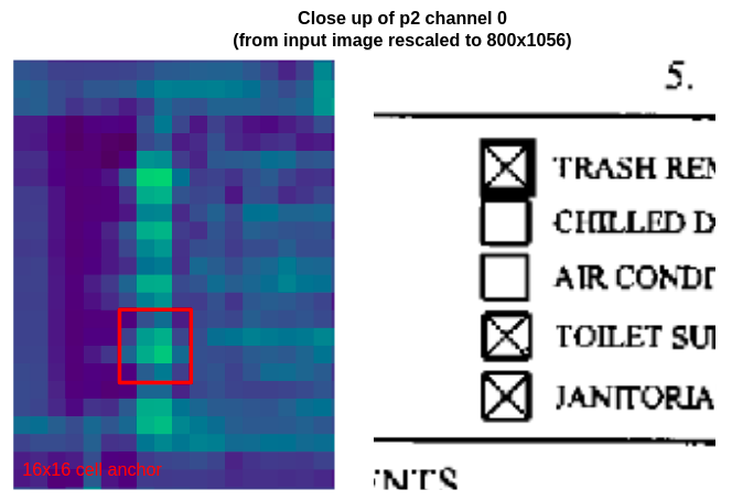
Close up of the second column of checkboxes on channel 0 of p2, the highest resolution feature map. The smallest cell anchor size (32x32 pixels, so 8x8 pixels on p2) is drawn in red for size comparison.
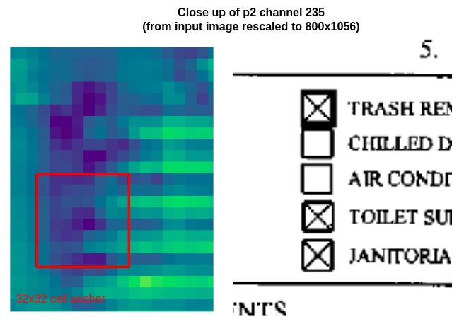
Close up of the second column of checkboxes on channel 235 of p2, the highest resolution feature map. The smallest cell anchor size (32x32 pixels, so 8x8 pixels on p2) is drawn in red for size comparison.
These images show that the smallest anchor size is significantly bigger than the checkbox feature representation, so the model has to learn a large regression change to fit the checkbox. Furthermore, at this resolution, the checkboxes appear as roughly 2x2 cell areas, so there is not enough detail to discriminate between filled and unfilled checkboxes.
6.2 Increase Image Resoluton
Increasing the image resolution allows more detail to be captured in the feature maps.
I changed the DataMapper image transform to
[ResizeShortestEdge(short_edge_length=(1600,), max_size=2666, sample_style='choice')]
This means the image is rescaled to double the default size (note: for the all documents dataset, I set max_size to 2071 so that images with certain ratios would not cause CUDA out of memory issues). I also disabled the RandomFlip (horizontal flip transform) because it is less applicable for document images.
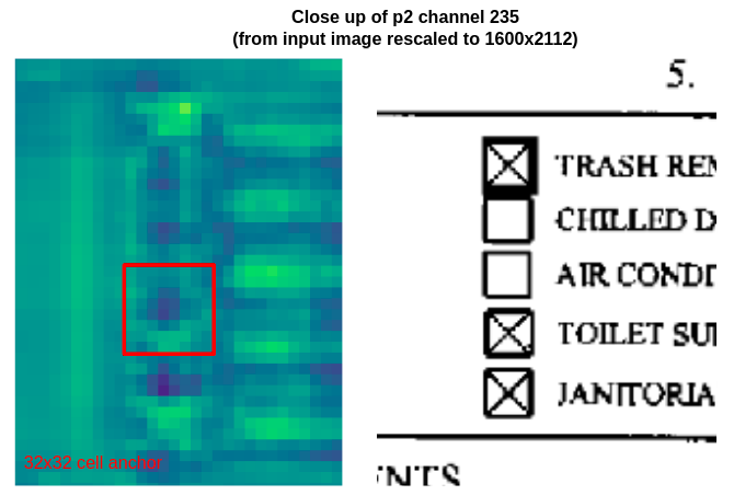
Close up of the second column of checkboxes on channel 235 of p2, the highest resolution feature map. The smallest cell anchor size (32x32 pixels, so 8x8 pixels on p2) is drawn in red for size comparison.
The checkboxes are represented in higher resolution, so it is slightly easier to discern filled vs. unfilled checkboxes. The cell anchor regression box is also closer to the expected checkbox size, so learning the regression parameters should be simpler.
Room for Improvement: Instead of just one number (1600,) the data transform could include a range of train-time resize transformations (as the default does). This would allow the model to learn features and proposals at a variety of different scales.
6.3 Add Smaller Anchor Size
Adding a smaller anchor size does not help with feature resolution, but it could improve recall for smaller classes since the regression parameters are simpler and matching proposals to ground truth by intersection over union (IoU) during training should work better.
I added a 16 cell anchor size to the model configuration.
MODEL.ANCHOR_GENERATOR.SIZES = [[16, 32, 64, 128, 256, 512]]
Close up of the second column of checkboxes on channel 235 of p2, the highest resolution feature map. The smallest cell anchor size (16x16 pixels, so 4x4 pixels on p2) is drawn in red for size comparison.
On the highest resolution feature map (p2), the smallest cell anchor (size 16) fits a single checkbox much better.
6.4 Results
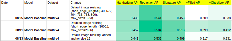
Each model was trained on the Lease-PNG dataset label set v4 and evaluated on the test split.
Inference Times: For an image resized by the default DataMapper, inference takes 0.067 sec / img. For an image double the default resize, inference takes 0.172 sec / img, or roughly 7x longer than inference on an image with the default resize transform.
Results on Multi-Label Model
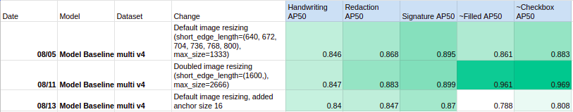
Per Class Average Precision 50 for multi-label models (Modified Binary COCOEvaluator). *For single-label v1 model overall AP50 = 0.838
![Per Class Average Recall for multi-label models (Modified Binary COCOEvalulator) *For single-label v1 model overall (AR) @[ IoU=0.50:0.95 | area= all | maxDets=100 ] = 0.502](/projects/handwriting-detection-with-faster-r-cnn-plus-experiments/img/eval_AR_multi_detect_smaller_objects.png)
Per Class Average Recall for multi-label models (Modified Binary COCOEvalulator) *For single-label v1 model overall (AR) @[ IoU=0.50:0.95 | area= all | maxDets=100 ] = 0.502
Per Class Average Precision for single- and multi-label models (Modified Binary COCOEvaluator and COCOEvaluator)
Looking at AP, AP50, and AR metrics for the multi-label models, doubling the image resize resulted in a slight improvement across all classes, especially across “Filled” and “Checkbox” classes. Adding the cell anchor size 16 did not noticeably improve the metrics.
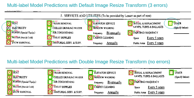
Predictions on LAK07176-Lease-a_Z-0.png with the default image resize transform (top) compared to the doubled image resize transform (bottom). With the default image resize transform the model missed a checkbox completely, and twice marked an unfilled checkbox as “Filled”. With the doubled image resize transform, the model did not make those errors.
Results on Single-Label Model
Average Precision (COCOEvaluator)
Average Recall (COCOEvaluator)
Per Class Average Precision (COCOEvaluator)
The single-label model was already performing well on the smaller classes. Doubling the image resize transform did not lead to a great improvement. I found this interesting, as the single-label models and multi-label models share the same Backbone network.
7 TEST ON OUT-OF-DISTRIBUTION DATA
Taking a model trained on one dataset and testing it on out-of-distribution (OOD) dataset is one way to sense how robust the model is.
The best performing model (in terms of both metrics and inference time) was the baseline single-label model with default transforms. In this evaluation, I took the best performing model trained on Lease PNGs and evaluated its predictions on FCC PNGs dataset.
7.1 Results
Per Class Average Precision (COCOEvaluator) – evaluated on the full FCC dataset
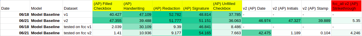
The “Signature” and “Date” classes performed very well on this OOD test. Given this performance, the “Date” class was included in the final label set (v5).
8 TRAIN FINAL ALL_DOCUMENT MODEL
The best performing model was the single-label baseline model (pre-trained on ImageNet and COCO) with default image resize transformations and cell anchors. The final model was trained on the all_doc dataset with v5 label set for 50,000 iterations.
8.1 Results
Average Precision (COCOEvaluator)
Average Recall (COCOEvaluator)
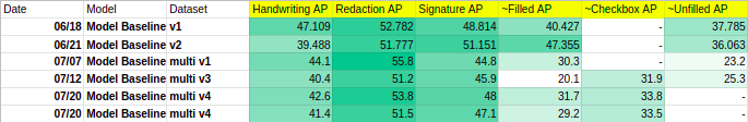
Per Class Average Precision (COCOEvaluator)
The evaluation metrics from the final model (last row) have been placed on the same table as the model baseline v1, model baseline v2, and the runs tested on OOD FCC PNGs data, for comparison. The final model performs unusually badly (numbers <10) on most classes, especially Filled and Unfilled Checkbox. It also seems to do somewhat poorly (numbers ~20) on Signature, Date, and Handwriting Detection. The only class it retains good performance on is Redaction.
8.2 Train-Validation Loss Curve
Given a poorly performing model, the first step in analysis is identifying whether the model is over-fitting or under-fitting. This can be accomplished by plotting the train and validation loss over model iterations.
I had run a custom train hook to evaluate the model on the test split every 2000 steps and log the validation loss (the hook ran 25 times, performed inference on ~500 images each time, overall adding ~2 hours to the total training time). The train and validation loss both steadily decreased and leveled off over the course of training.
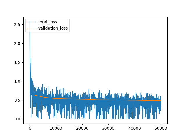
Total Loss vs. Validation Loss from training all_doc model on 50,000 iterations
Resources
- How to use TensorBoard with PyTorch — PyTorch Tutorials 1.9.0+cu102 documentation
- Training on Detectron2 with a Validation set, and plot loss on it to avoid overfitting
9 QUALITATIVE AND QUANTITATIVE ANALYSIS OF CLASS CONFUSION
It is very useful to analyze a model’s error modes, especially class confusion, false positives, and false negatives. I wrote a script to create a object-detection confusion matrix to identify class confusion and unpaired predictions and ground truths, and visualizing high and low confidence predictions by prediction label and ground truth label.
I’ll focus this analysis on the test split predictions from the single-label models trained on
- Lease-PNG label set v1 with default transform
- Lease-PNG label set v1 with doubled image resize transform
- Lease-PNG label set v2
- All_Docs label set v5
To create the object-detection confusion matrices, I first created a pairwise IoU matrix between all the predictions and the ground truth bounding boxes for each image. I discarded pairings with an IoU less than the threshold (0.5) and then matched each prediction with the ground truth it has the most IoU with. In this way, predictions can be matched with 1 or 0 ground truths, and ground truths can be matched with any number of predictions. The confusion matrix indicates whether the prediction’s label agrees with the closest ground truth’s label or if there is class confusion. If a prediction has no closest ground truth (no IoU > threshold) then it is counted in the unmatched column. If a ground truth has no matches with predictions, then it is counted in the unmatched row.
Then, to get a better visual sense of error modes, I made panels that visualized the predictions in terms of predicted label vs. ground truth label and ordered instances by model confidence. If the pairing had less than or equal to 100 predictions, I displayed all of them. If it had between 100 and 200 predictions, I displayed an evenly indexed range of predictions based on confidence value order. If it had more than 200 predictions, I displayed the top 100 high confidence and bottom 100 low confidence predictions. After examining these panels, I marked the potential real cases of class confusion in red text on the confusion matrices tables.
9.1 Performance on Lease-PNG label set v1
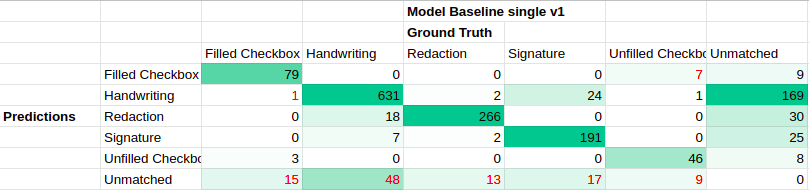
confusion matrix for single-label model baseline trained on Lease-PNG label set v1 with default transform
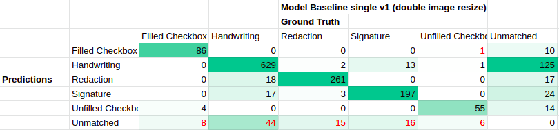
confusion matrix for single-label model baseline trained on Lease-PNG label set v1 with doubled image resize transform
These confusion matrices were created from model predictions on the Lease PNG label set v1’s test set. The confusion matrices for the model baseline with default transform images and the model baseline with double image resize transform predictions both look pretty similar. Both have strong agreement between prediction labels and ground truth labels (high counts on the diagonal), and do a decent job detecting Filled Checkboxes and Unfilled Checkboxes (a small portion of checkbox ground truths are unpaired, the model with doubled resized images does slightly better here). In terms of undesirable behavior, both have many unmatched predictions that did not overlap with any ground truths (especially for the Handwriting class), a scattering of predictions with class confusion, and a small number of unmatched ground truths that did not overlap with a prediction (especially for the Handwriting class).
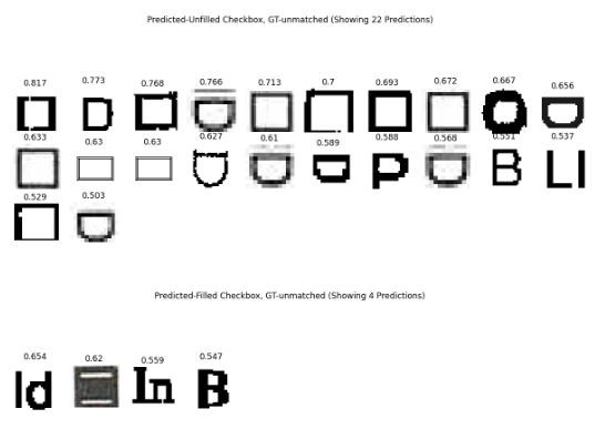
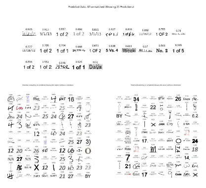
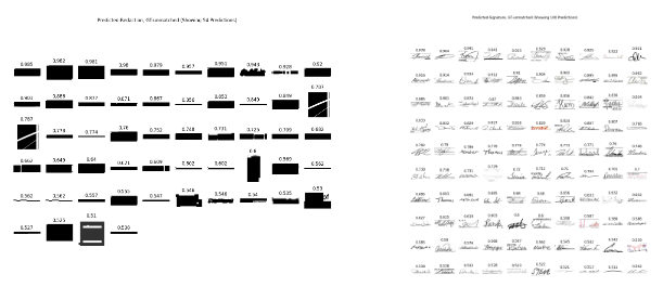
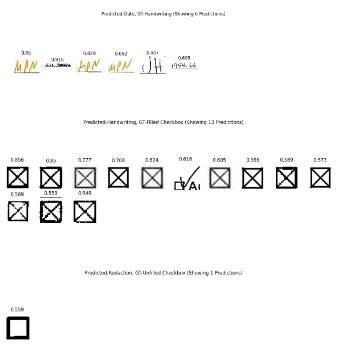
Unmatched Predictions Visualized
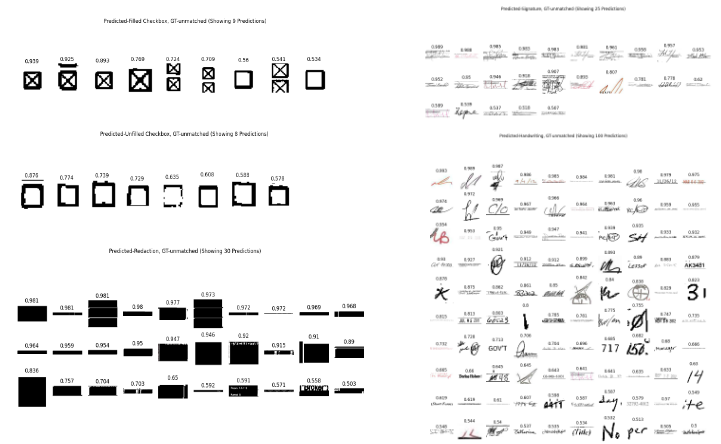
Unmatched predictions from model baseline with default transform: Predicted-Filled Checkbox (top-left), Predicted-Unfilled Checkbox (middle-left), Predicted-Redaction (bottom-left), Predicted-Signature (top-right), Predicted-Handwriting (bottom-right)
For the model baseline with default transform’s predictions, the vast majority of predictions not matching a ground truth seem to be correctly predicted, but missing ground truth labels. For the unmatched “Redaction” class, there are maybe 6 instances where white text on a black background has been predicted as Redaction. Overall, no real problems. Three of the unmatched “Filled Checkboxes” may have been unmatched due to the predicted bounding box covering the area of two checkboxes (and thus likely exceeding the 0.5 IoU threshold).
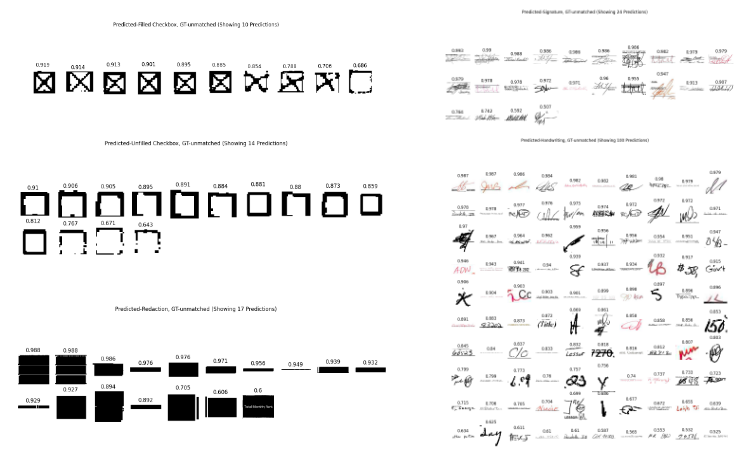
Unmatched predictions from model baseline with doubled image resize transform: Predicted-Filled Checkbox (top-left), Predicted-Unfilled Checkbox (middle-left), Predicted-Redaction (bottom-left), Predicted-Signature (top-right), Predicted-Handwriting (bottom-right)
Like the model with default transform, the vast majority of predictions not matching a ground truth seem to be correctly predicted, but missing ground truth labels. The issue where three of the predicted “Filled Checkboxes” had too large bounding box areas has gone away, indicating that the bounding box regression was likely more successful on the larger images.
Class Confusion Visualized
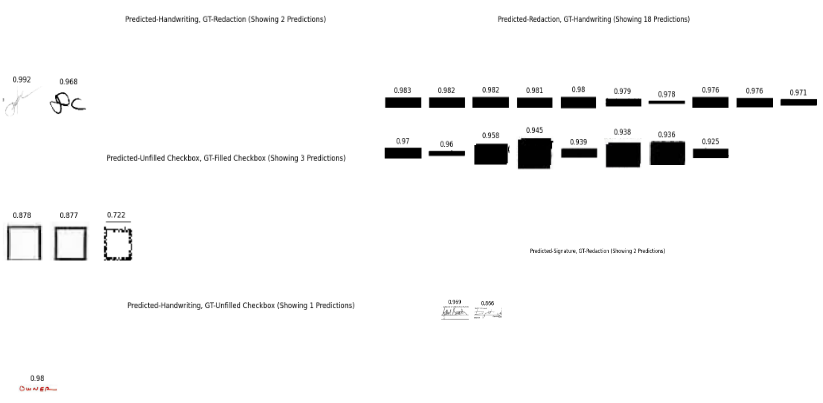
Incorrectly marked class confusion from model baseline with default transform: Predicted-Handwriting:GT-Redaction (top-left), Predicted-Unfilled Checkbox:GT-Filled Checkbox (middle-left), Predicted-Handwriting:GT-Unfilled Checkbox (bottom-left), Predicted-Redaction:GT-Handwriting (top-right), Predicted-Signature:GT-Redaction (bottom-right).
In terms of class confusion, there is very little. For all the predictions in pairings of Predicted-Handwriting:GT-Redaction (2), Predicted-Unfilled Checkbox:GT-Filled-Checkbox (3), Predicted-Handwriting:GT-Unfilled Checkbox (1), Predicted-Redaction:GT-Handwriting (18), and Predicted-Signature:GT-Redaction (2), the ground truth label is wrong and the predicted label is right.
Real and potentially real class confusion form model baseline with default transform. From top to bottom: Predicted-Handwriting:GT-Filled Checkbox, Predicted-Filled Checkbox:GT-Unfilled Checkbox, Predicted-Signature:GT-Handwriting, Predicted-Handwriting:GT-Signature
Aside from a single Filled Checkbox predicted as Handwriting and 7 Unfilled checkboxes predicted as Filled, there is no obvious class confusion. The class confusion between Handwriting and Signature class may exist. Without additional context clues, all 7+24 instances of this confusion look like they could be either Signatures or messily/cursive Handwritten names.
9.2 Performance on Lease-PNG label set v2
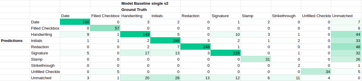
confusion matrix for single-label model baseline trained on Lease-PNG label set v2 with default transform
This confusion matrix reveals some of the reasons behind poor AP performance for certain classes, namely that Stamp and Unfilled Checkbox had ~40 predictions to be evaluated on, and Strikethrough did not even detect most of the ground truth strikethrough instances.
In terms of desired behavior, the model did very well on detecting the other classes, especially the small checkbox classes (high counts on the diagonals and very few instances of class confusion or unmatched ground truths).
9.3 Performance on All_Docs label set v5 (Final Model)
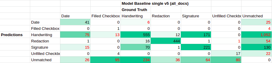
confusion matrix for single-label model baseline trained on All_Docs label set v5 with default transform
The final document model, trained on the all documents dataset using label set v5 for 50k iterations, had a pretty bad looking confusion matrix. In particular, almost all the Filled Checkbox and Unfilled Checkbox failed to be detected.
All Doc document image (0003f6ad-e10a-9b4a-3d73-9d387656d39c-1.png) as an example of predictions missing the clean checkboxes in the center row of the page.
The confusion matrix also indicates several unmatched Handwriting predictions, some unmatched Filled Checkboxes and Unfilled Checkboxes, and class confusion between Handwriting and Date, Unfilled Checkbox and Date, and Handwriting and Filled Checkbox.
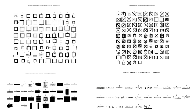
Unmatched Predictions Visualized
Unmatched predictions for Unfilled Checkbox (top) and Filled Checkbox (bottom)
The unmatched predictions for the checkbox classes seem to be picking up on circular letters and semi-circle shapes.
Unmatched predictions for Date (top), high confidence Handwriting (top-left) and low confidence Handwriting (bottom-right)
The unmatched predictions for Date and Handwriting all seem to be picking up on numbers. Date in particular has lots of instances of page numbers, as well as text on a messy grey background. The Handwriting predictions seem to pick up on standalone numbers, as well as X marks and stamped or unusual font text.
Unmatched predictions for Redaction (left) and Signature (right)
The unmatched predictions for Redaction and Signature seem to be pretty correct. The model might be predicting redaction in areas with dark backgrounds and not real redaction, so a closer look at the predictions in the context of their document may be needed for validation.
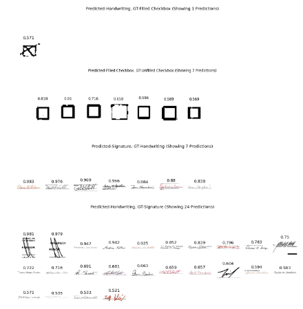
Class Confusion Visualized
Class confusion when GT-Date is predicted as Handwriting (top) and Signature (bottom)
The biggest class confusion is when visually obvious Date instances are predicted as Handwriting or Signature.
Class confusion when GT-Handwriting predicted as Date (top), when GT-Filled Checkbox predicted as Handwriting (middle). Single instance when GT-Unfilled Checkbox was predicted as Redaction (bottom).
There is also some consistent class confusion when slanted initials in the Handwriting class are predicted as Date, or X-shaped or check-shaped marks in Filled Checkboxes are predicted as Handwriting.
Unmatched Ground Truths Visualized
Unmatched ground truths: GT-Unfilled Checkbox (top-left), GT-Redaction (bottom-left), GT-Filled Checkbox (top-right), GT-Date (bottom-right)
There is some variance and messiness in the missed ground truths, but not overwhelmingly so. They might have been detected at a confidence lower than the 0.5 threshold? It is interesting that many of these checkboxes come from Lease PNG documents that the previous models could predict fine on.
10 FUTURE WORK
10.1 Analysis of Prediction Bounding Box Overlap
Work could be done to measure and limit overlapping bounding boxes. The Faster-R-CNN model seems to permit overlapping bounding boxes in two cases:
- Instances of the same class if the instances have less than 0.5 overlap (this evades the ROIHead per-class non-maximal suppression threshold)
- Instances of different classes on the same area (this might be evading the Region Proposal Network non-maximal suppression threshold)
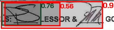
Example of Overlapping Signature Predictions (same class, less than 0.5 overlap)
Example of Overlapping Handwriting and Signature Predictions (different classes, same area)
10.2 Reduce False Positives with Explicit Labeling
As seen in the all_doc model’s unmatched predictions, there are some recurring false positives, such as page numbers, numbers in general, dark backgrounds, and curvy letters or X marks in unusual fonts. One may be able to teach the model to filter out false positives by explicitly labeling those as another class.
10.3 Reduce Inference Time and Memory Usage
The default single-label Faster R-CNN model is rather slow and consumes a lot of memory. It takes ~5 minutes to run inference on ~500 documents. Due to its memory requirements, training it on the dev cluster failed a couple of times.
One potential solution to the memory issue is gradient check-pointing, which is a method used for reducing the memory footprint when training deep neural networks, at the cost of having a small increase in computation time.
10.4 Find Out Why All_Docs Model Performed Poorly on Checkbox Detection
The final all_docs model trained on all the documents struggled to detect Filled Checkboxes and Unfilled Checkboxes, even on documents from the Lease PNG dataset.
11 APPENDIX: FASTER-RCNN IMPLEMENTATION DETAILS
A large portion of my internship involved understanding how Faster-RCNN worked. In hopes of helping future me (and others) with this task in the future, I have placed my clean and organized notes here.
DataMapper
The DataMapper applies transformations to input images. By default, it rescales the images so they are smaller (so shortest edge is a random choice of (640, 672, 704, 736, 768, 800)), and flips images horizontally.
[ResizeShortestEdge(
  short_edge_length=(640, 672, 704, 736, 768, 800),
  max_size=1333,
  sample_style='choice'),
  RandomFlip()
  ]
Backbone Network
The backbone network receives a transformed input image from the Data Mapper and creates feature maps at various scales by using a Feature Pyramid Network (FPN) and a ResNet. By default, it creates feature maps using 5 strides (S = 4, 8, 16, 32, and 64) called p2, p3, p4, p5, and p6. Each feature map has 256 channels.
Details on Feature Pyramid Network
The Feature Pyramid Network is an accurate and fast feature extractor that replaces the default feature extractor of Faster R-CNN. It is composed of a bottom-up pathway (ResNet convolution network for feature extraction) and a top-down pathway (lateral connections for merging high-level semantic features information into lower feature maps to create higher resolution layers)
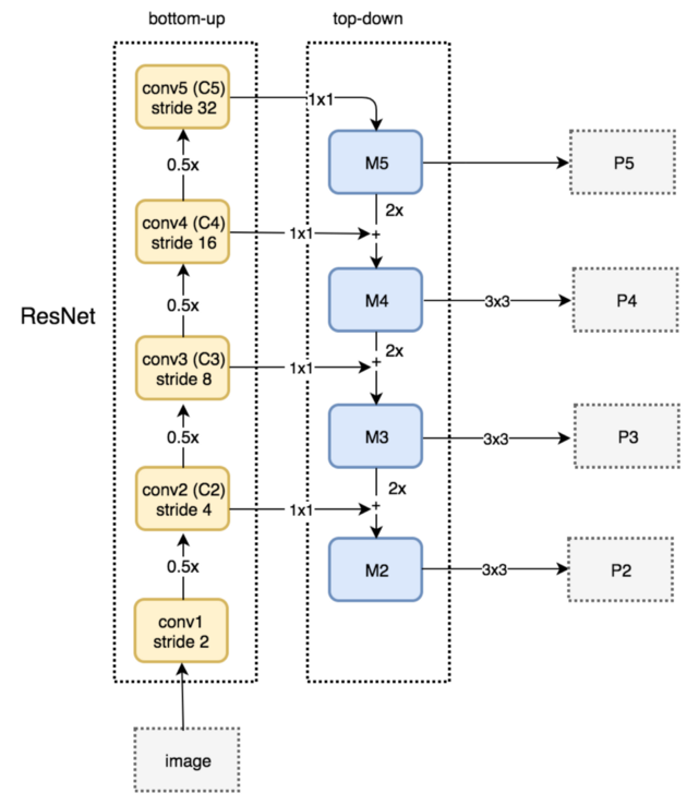
Feature Pyramid Network top-down and bottom-up pathway. (Source: Understanding Feature Pyramid Networks for object detection (FPN))
Region Proposal Network (RPN)
The RPN associates the backbone network’s feature maps to ground-truth box locations, uses a binary classifier to determine “objectness score” over the feature maps, and outputs box proposals of regions that probably contain an object. This is where anchors, ground truth locations, and the “objectness” loss functions come into play.
RPN Head
The RPN uses a convolutional neural network (RPN Head) that takes feature maps and ground truth box locations as its inputs. Then it outputs pred_objectness_logits and pred_anchor_deltas.
For each level of feature map (p2, p3, p4, p5, p6) the RPN Head calculates:
pred_objectness_logits(B, 3 ch, Hi, Wi): probability map of object existencepred_anchor_deltas(B, 3×4 ch, Hi, Wi): box shape relative to anchors
B stands for batch size, Hi and Wi are height and width of the feature map, and the 3 channels correspond to the three potential classes (“foreground”, “background”, and “ignore”).
During training, a loss function is used to determine how close RPN Head objectness predictions are to the ground truth boxes. To compare the pred_objectness_logits map and pred_anchor_deltas map to the ground truth boxes, the ground truth boxes have to be mapped to the feature maps.
Map Ground Truths to Feature Maps With Cell Anchors (during training)
The cell anchor generation step creates objectness_logits (ground truth objectness map) and anchor_deltas (ground truth anchor deltas map) with values at each grid point of the feature map.
## MODEL.ANCHOR_GENERATOR.SIZES = [[32], [64], [128], [256], [512]]
## detectron-v2 applied all the cell anchors to all the feature maps
MODEL.ANCHOR_GENERATOR.SIZES = [[32, 64, 128, 256, 512]]
MODEL.ANCHOR_GENERATOR.ASPECT_RATIOS = [[0.5, 1.0, 2.0]]
The five elements of the ANCHOR_GENERATOR.SIZES list correspond to five levels of feature maps (P2 to P6). If len(ANCHOR_GENERATOR.SIZES) == 1, then the size ANCHOR_GENERATOR.SIZES[0] cell anchors are applied to each feature map.
Each cell anchor is applied at each grid point of the feature map at each aspect ratio. For example P2 (stride=4) has one cell anchor whose size is 32, so its anchors cover 4x16 cells, 8x8 cells, and 16x4 cells of the p2 feature map, which translates to regions of 22.6x45.2 pixels, 32x32 pixels, and 45.2x22.6 pixels on the transformed input image).
Once the anchors are generated, objectness_logits can be calculated. First, the intersections between all the generated anchors and all the ground truth boxes are calculated in a Intersection-over-Union (IoU) Matrix. Generated anchors with intersection greater than 0.7 are labeled foreground (“1”), less than 0.3 are labeled background (“0”), and in between (0.3 < x < 0.7) are labeled ignored (“-1”).
MODEL.RPN.IOU_THRESHOLDS = [0.3, 0.7]
MODEL.RPN.IOU_LABELS = [0, -1, 1]
Then anchor_deltas are calculated as the regression parameters (Δx, Δy, Δw, and Δh) between each foreground box and its closest ground truth box.
Loss Function (during training)
Since the majority of generated anchors are going to be of the “background” class, the labels are re-sampled to fix the imbalance and make it easier to learn foreground classes. Then two loss function are applied:
- Objectness Loss: Binary cross entropy loss comparing
pred_objectness_logitsto foregroundobjectness_logits - Localization Loss: L1 loss comparing
pred_anchor_deltasto foreground and backgroundanchor_deltas
Box Proposal Selection
The RPN applies the pred_anchor_deltas, sorts the predicted boxes by pred_objectness_logits, chooses the top 2,000 boxes from each feature level, applies non-maximum suppression at each level independently, and keeps the surviving 1,000 top-scored region proposal boxes.
ROI Head
The ROI Head is a multi-class classifier that receives the backbone network’s feature maps (p2, p3, p4, and p5 – p6 is not used), the RPN’s box proposals (1,000 top scoring proposal boxes, their objectness_logits are not used), and the ground truth boxes.
Re-Sampling and Matching (during training)
Ground truth boxes are added to the 1,000 RPN boxes. Then the IoU matrix is calculated between the box proposals and the ground truth (with proposals labeled as foreground if they have greater than 0.5 IoU and background otherwise; the added ground truths match themselves perfectly). Finally, the group is re-sampled to balance the proportion of foreground and background proposal boxes.
Cropping
The ROI pooling process uses the coordinates of the proposal boxes to crop the corresponding rectangular regions of the feature maps. It uses a level assignment rule to determine which feature map the region of interest (ROI) should be cropped from (ex: the small boxes should crop from p2, big boxes from p5).
## Eqn.(1) in FPN paper
    level_assignments = torch.floor(
        canonical_level + torch.log2(box_sizes / canonical_box_size + eps)
    )
Here eps=4, canonical_box_size=224. So if the proposal box was 224x224, it would be assigned to p4.
In order to accurately crop the ROI by the proposal boxes which have floating-point coordinates, a method called ROIAlign has been proposed in the Mask R-CNN paper. In Detectron 2, the default pooling method is called ROIAlignV2, which is the slightly modified version of ROIAlign.
Box Head
The Box Head (FastRCNNConvFCHead) classifies the object within the region of interest and adjusts the box’s position and shape. It consists of linear fully-connected (FC) layers and two final box_predictor layers that project the output into a scores tensor (B, 80+1) and a prediction deltas tensor (B, 80x4). In the original ImageNet dataset, there were 80 classes. The “+1” final position indicates the background class.
Loss Calculation
Two loss functions are applied:
- Classification Loss: Softmax cross entropy loss comparing prediction scores to ground truth class indexes.
- Localization Loss: L1 loss comparing
pred_proposal_deltasto foregroundgt_proposal_deltas
Inference
Just like in the RPN, to get the final output, the ROIHead applies the prediction deltas to get the final box coordinates, filters out low-scoring boxes, uses non-maximum suppression, and returns the top-k results.