Understanding the geometric intuition and algorithms for solving linear programming problems. Covers (1) defining the solution space as the area within a convex polytope space, (2) understanding that the optimal solution occurs at a vertex point and translating that geometric intuition and more efficient search path into the Simplex matrix-based algorithm, (3) the idea of Duality and how it exposes additional information, and (4) how the Interior Point method works not just for linear programs, but also for more general convex optimization problems.
Table of Contents
Purpose
Linear Programming: method for solving system of linear inequalities efficiently.
Real-life Examples
- Allocate optimal staff positions based on worker scores
- Allocate optimal manufacturing products based on resource cost
- Allocate optimal menu based on cost and nutrition needs
- Network flows, game theory, transportation, production, economics
Set-Up
- Given decision variables (i.e. $x_1$, $x_2$, …, $x_3$)
- Given linear objective equation (i.e. optimization equation)
- Given system of linear constraints
- Find maximal value of linear objective equation
2-variable example ($x$, $y$) $$\displaylines{ &\text{max } &3x + 4y \\ &\text{subject to } &x + 2y&\le 14 \\ &&-3x + y &\le 0 \\ &&x - y &\le 2 \\ &&0 \le x, y }$$
3-variable example ($x_1$, $x_2$, $x_3$) $$\displaylines{ &\text{max } &5x_1 + 4x_2 + 3x_3 \\ &\text{subject to } &2x_1 + 3x_2 + x_3 &\le 5 \\ &&4x_1 + x_2 + 2x_3 &\le 11 \\ &&3x_1 + 4x_2 + 2x_3 &\le 8 \\ &&0 \le x_1, x_2, x_3 }$$
Limitations & Assumptions
Infeasible solution spaces
Linear programs are not solvable when the solution space spills into infinity or does not form a convex polytope solution space (i.e. a side of polyope is not closed because constraint hyperplanes are parallel or there are not enough constraint hyperplanes).
Assume standardized form
Maximize objective function
- if minimize, negate coefficients
All constraints must be $\le$ constraints
- if $a \ge b$ then negate as $-a \le -b$
- if $a = b$ then define as inequality $a \le b$ AND $-a \le -b$
Decision variables, slack variables, and objective value must be non-negative ($\ge 0$)
- if $z = a - b$ then $a, b \ge 0$
Summary of Intuitive Tips and Tricks
V1 (Graphing). Define the solution space as the area within a convex polytope space
For linear programs, a feasible solution set exists as the points within the convex polytope formed by the inequality constraints’ hyperplanes. Convex means that a line between any two points within shape lies within the shape. Convex optimization problems have the following useful properties:
- Every local minimum is a global minimum
- The optimal solution set is convex
- If the objective function is strictly convex, then problem has at most one optimal point
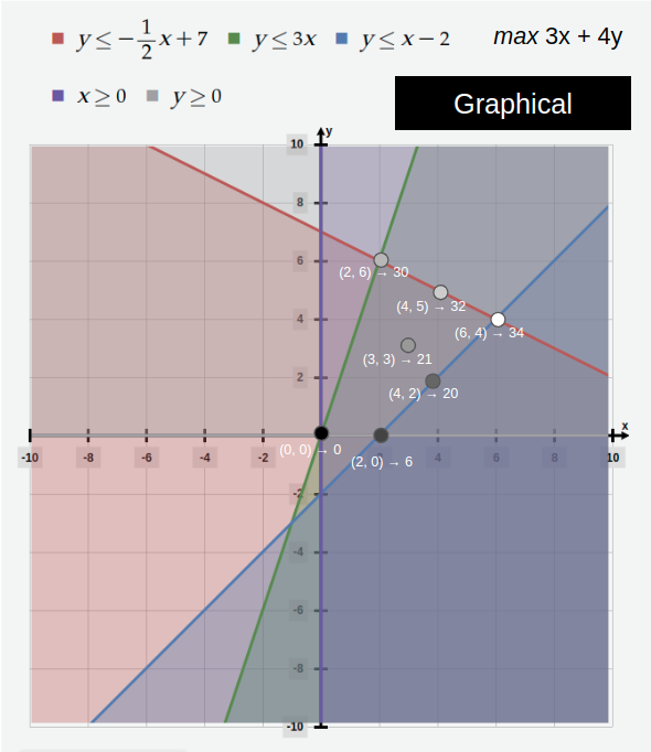
Graphical approach to finding the maximum value of the objective function.
The objective function has a fixed slope and a variable intercept, so the optimal solution can be found by path-finding toward the local maximum within the solution space.
V1 → V2 (Slackness). Narrow the solution space to a finite set of vertex points
Note that if the optimal solution exists within the convex polytope solution space, then it must be on a extreme (vertex) point (i.e. pathfinding through the valid space will always go towards a vertex as a min or max value; visual proof). A convex polytope has a finite number of extreme points. To coerce a system of linear constraints into a system of vertices, turn the constraints into equalities using slack variables.
V2 → V3 (Simplex). Search for optimal point without traversing the entire set of vertices
If the starting vertex is not the maximum point, then it has at least one edge leading to another vertex such that the objective function is strictly increasing along that edge (visual proof). To find the maximum, first pick a vertex, then continually jump to neighboring vertex points with higher objective values. This will eventually lead to a vertex with no neighbors having higher objective values. The Simplex Algorithm can use steps from Gaussian Elimination to turn the geometric intuition into a matrix system of equations.

Simplex Algorithm approach to finding the maximum value of the objective function.
The process of stringing together a sequence of simplex pivots in order to locate an optimal solution is called the Simplex Algorithm. It was discovered by George Dantzig (1914-2005). The Simplex Algorithm is considered one of the ten most important algorithmic discoveries of the 20th century. Even with after the discovery of the Interior Point Methods, for many specially structured linear programming problems, the Simplex remains the most efficient algorithm.
V3 → V4 (Duality). View a process from two perspectives to expose additional information
Any activity has two effects. For example, from an economics perspective, a transaction to buy equipment has to be recorded twice: (1) it increased asset because production increased, and (2) it decreased asset because resources decreased. The primal problem is the original maximization problem, the dual problem is the corresponding resource cost minimization problem.
Linear programming problems meet the conditions for Strong Duality, which states that any optimally weighted action equally balances both effects, so any optimal tableau simultaneously gives optimal solutions to both the primal and dual problems. Taking advantage of this computational efficiency is important for both linear programming duality theory and sensitivity analysis. Solving the dual problem has three important outcomes:
- Finds the marginal worth of an additional unit of any of the resources
- Finds the opportunity cost of allocating resources to one activity relative to other activities after pricing activities using marginal worths
- Enables quick checking of work (do not redo calculation, instead check the scaling factor)
V4 → V5 (Interior Point). Fewer iterations than Simplex, gradient-based approach that follows a central path
The Simplex method starts out with maintaining complementary slackness and a basic feasible solution for the primal problem, and then tries to solve the dual problem in order to find the optimal basic feasible solution. Perfectly solving the dual solution takes a low computation cost per iteration and can take many iterations. At best case, the Simplex Algorithm takes a polynomial number of iterations (to number of constraints), and at worst case takes an exponential number of iterations (to number of variables).
Interior Point methods achieve a better time complexity by starting out being both primal and dual feasible and working towards complementary slackness. The Interior Point methods require $O(\sqrt{n}\log(1/\epsilon))$ iterations (worst case polynomial time complexity) to get a primal-dual solution that is feasible and optimal up to some tolerance measured by $\epsilon$. Thus, the Interior Point methods takes fewer iterations to solve, but require larger computational cost per iteration.
In essence, the Interior Point methods work by path-finding along a central path that starts from the analytical center of the convex solution space and heads towards the optimal solution, always staying within the interior of the convex solution space (visual proof). The larger computational cost per iteration results from playing a min-max game on the Lagrangian of the Dual. It can use an unconstrained convex approximation solver (i.e. Newton’s Method) to power its approximation logic steps in a matrix-oriented way.
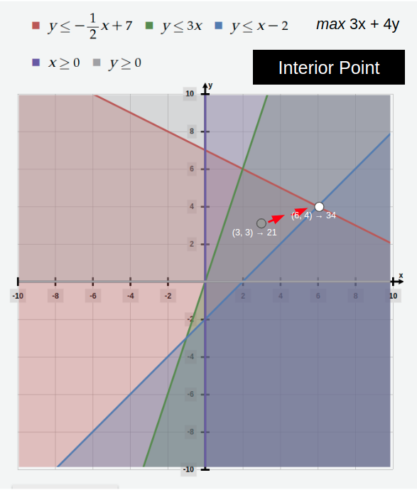
Interior Point Methods approach to finding the maximum value of the objective function.
The Interior Point Method was published by Narendra Karmarkar in 1984. This approach works for convex optimization problems, so it also works for problems beyond the realm of linear programming.
V1. Encode Graphical Approach
- Plot system of linear constraints
- Choose valid point that maximizes objective
2-Variable Toy Example ($x = x_1$, $y = x_2$)
# plot constraint inequalities
y <= 7 - x/2
y <= 3x
y >= x - 2

# plot objective equation
objective: 3x + 4y
V2. Encode Complementary Slackness
- For each constraint: convert to standard form, add non-negative slack variables
- Solve the system of linear equations (i.e. using Gaussian Elimination)
Continuing with 2-Variable Toy Example ($x = x_1$, $y = x_2$)
# convert constraint inequalities to standard form
x   +   2y  <=  14
-3x +   y   <=  0
x   +   -y  <=  2
-x, -y <= 0

# add slack variable (w1, w2, w3) to each constraint
# turn inequality into an equality (vertex points)
        x   +   2y  +   w1          =   14
        -3x +   y       +   w2      =   0
        x   +   -y          +   w3  =   2
# objective function
-z  +   3x  +   4y                  =   0
# make sure all variables are non-negative
-z, -x, -y, -w1, -w2, -w3 <= 0

# solve system of linear equations
V3. Encode Simplex Algorithm
- Translate geometric intuition into computation-friendly algorithms
- “Simplex” means the simplest possible polytope in any given space.
- The process of moving from one basic feasible solution (analogous to vertex) to the next is called a simplex pivot.
Part A: convert standard form to matrix representation
Objective value ($z$):
- Let $z$ be the variable referring to the objective value
- Let $x$ be a vector containing the variables to optimize
- Express the linear objective as $z = c^\intercal x$ where $c$ is a vector containing the coefficients of the variables
Constraints ($Ax \le b$):
- Express constraint $i$ as $a_i^\intercal x \le b_i$ where $a_i$ is a vector containing the coefficients of the constraint and $b_i$ is a constant.
- Let $A = [a_1, a_2, … a_3]^\intercal$ be a matrix with each vector $a$ as row $i$, so the system of constraint equalities become $Ax \le b$.
- Requiring that $x \ge 0$ gives
$$\displaylines{ &\text{maximize } & z = c^\intercal x \\ &\text{subject to } &Ax \le b \\ &&x \ge 0 }$$
Add slack variables ($w$)
- Redefine $x$ be a vector containing the variables to optimize and the slack variables: $x = [x_1, x_2, …, x_3, w_1, w_2, …, w_3]$
- Note how the slack variable coefficients form an identity matrix ($I$)
$$\displaylines{ &\text{subject to} & 0z + \begin{bmatrix} A & I\end{bmatrix} x = b \\ &\text{objective} & -z + \begin{bmatrix} c^\intercal & 0\end{bmatrix} x = 0 \\ &&z, x \ge 0 }$$
The values of $A$, $I$, $b$, $-1$, $c^\intercal$, and $0$ are known. The optimal values of $z$ and $x$ are not known. The system written in block structured matrix notation is:
$$\begin{bmatrix} 0 & A & I \\ -1 & c^\intercal & 0 \end{bmatrix} \\ \begin{bmatrix} z \\ x \end{bmatrix} = \\ \begin{bmatrix} b \\ 0 \end{bmatrix}$$
Part B: convert matrix representation to canonical tableau form and a find basic feasible solution (choose starting vertex point)
This initial system defines the unknown slack variables $[w1, w2, …, w3]$ and unknown objective value $z$ as a linear combination of the unknown initial decision variables $[x1, x2, …, x3]$. Not including $z$, the variables “defined” in this way are called the basic variables, while the remaining variables are called non-basic variables.
- objective value: $z$
- non-basic variables: multiply with the columns of $A$ and $c^\intercal$
- basic variables: only multiply with the columns of the identity matrix ($I$).
Solving for an initial basic feasible solution, analogous to choosing the starting vertex of the concave polytope, can happen by setting the non-basic variables to zero. This boils down to setting the $\text{basic variables} = b$ and $z = 0$ because the system simplifies to: $$\displaylines{ (z * 0) + (A * 0) + (I * \text{basic variables}) = b \\ (z * -1) + (c^\intercal * 0) + (0 * \text{basic variables}) = 0 }$$
Continuing with 3-variable example
$$\displaylines{ &x_1 = 0 && w_1 = 5 \\ &x_2 = 0 & \text{gives} & w_2 = 11 \\ &x_3 = 0 && w_3 = 8 \\ &&& z = 0 }$$
Since the elements of vector $x = [0, 0, 0, 5, 11, 8, 0]$ are non-negative, the point lies in the feasible region of the solution space. In general, a solution of four linear equations defines three of the variables in $x$ in terms of the remaining three variables and has the same solution set as the initial system.
Part C: Pivot operation, similar to Gaussian elimination (move along edges to neighbor vertices with greater $z$ values)
The initial basic feasible solution is not optimal. To find a better value of $z$ (analogous to moving to the neighboring vertex, moving on an edge where the value of $z$ is strictly increasing), increase the value of one of the non-basic variables from its current value of 0.
This series of operations can be legibly expressed using a pivot table, which is simply a labeled version of the system matrix multiplication.
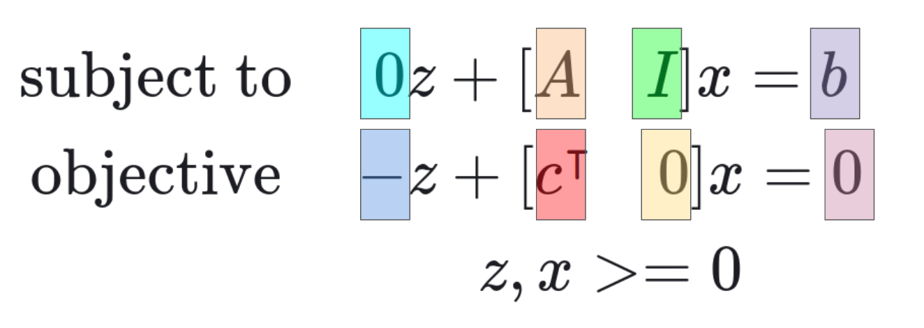
Colored matrix multiplication diagram.
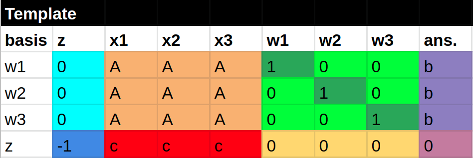
Colored pivot table set-up diagram. Note how the values for the initial basic feasible solution ($w1 = b$, $w2 = b$, $w3 = b$, and $z = 0$) appear in the ans. column.
Visual guide to using the pivot table to increase the value of $z$:
Written guide to using the pivot table:
Step 1: Fill in the pivot table according to the matrix multiplication pattern.
Step 2: Look at objective row, find biggest, most positive element. As a pivot, this will cause the largest increase in the objective function. Once the pivot column is chosen, the pivot row must must be chosen such that the solution is still feasible (choose a non-zero pivot element with the smallest ratio of $\text{ans}/\text{pivot column value}$. Choosing the smallest value ensures that all the values in the $\text{ans}$ (future BFS) stay positive after Step 3.
Step 3: Multiply pivot row by the reciprocal of the pivot element to make it $1$, then add multiples of the row to the other rows until all other entries in the pivot column are $0$. This transforms the column from a non-basic variable to a basic variable. It also replaces the corresponding variable in the identity matrix. The added and replaced variables are called entering and leaving variables respectively.
Step 4: Repeat Step 2 and Step 3 until the objective row has all zero or negative values. When this happens, no choice of pivot will maximize the objective (this corresponds to finding the final vertex on the polytope). The final BFS is in the $\text{ans}$ column.
V4. Encode Primal-Dual
- Every primal optimization problem has an associated dual
Definition of primal and dual problems
Primal problem definition $$\displaylines{ &\text{maximize } & z = c^\intercal x \\ &\text{subject to } &Ax \le b \\ &&x \ge 0 }$$
Dual problem definition $$\displaylines{ &\text{minimize } & z = b^\intercal y \\ &\text{subject to } &Ay \ge c \\ &&y \ge 0 }$$
By the Theorem of Strong Duality (holds for linear programming problems):
$$c^\intercal x = b^\intercal y$$
Continuing with 3-variable example
Problem: Cathy makes chairs, tables, and fences and wants to have as much money as possible.
- Primal: maximize marginal revenue
- Dual: minimize marginal costs
# given
activity    create_table :     2 wood and 4 hour and 3 coat per table
activity    create_chair :     3 wood and 1 hour and 4 coat per chair
activity    create_fence :     1 wood and 2 hour and 2 coat per fence

limit   price_table :   $5 per table
limit   price_fence :   $4 per fence
limit   price_chair :   $3 per chair

limit    limit_wood :   5 wood in stock
limit    limit_hour :   11 hour in stock
limit    limit_coat :   8 coats in stock

# product (primal)
find    num_table
find    num_chair
find    num_fence

# resources (dual)
find    price_wood
find    price_hour
find    price_coat
How do I optimally maximize the revenue when making products?
# primal: maximize marginal revenue (limited by resources)
z = 5 * num_table + 4 * num_chair * 3 * num_fence

# constraints for making products
2 * num_chair + 3 * num_table + 1 * num_fence <= 5 wood
4 * num_chair + 1 * num_table + 2 * num_fence <= 11 hour
3 * num_chair + 4 * num_table + 2 * num_fence <= 8 coat
num_table, num_chair, num_fence >= 0
$$\displaylines{ &\text{max } &5x_1 + 4x_2 + 3x_3 \\ &\text{subject to } &2x_1 + 3x_2 + x_3 &\le 5 \\ &&4x_1 + x_2 + 2x_3 &\le 11 \\ &&3x_1 + 4x_2 + 2x_3 &\le 8 \\ &&0 \le x_1, x_2, x_3 }$$
How do I optimally minimize resource cost when making products?
# Dual: minimize marginal cost (limited by product prices)
z = 5 * price_wood + 11 * price_hour + 8 * price_coat

# constraints for making products
2 * price_wood + 4 * price_hour + 3 * price_coat >= 5 price_table
3 * price_wood + 1 * price_hour + 4 * price_coat >= 4 price_chair
1 * price_wood + 2 * price_hour + 2 * price_coat >= 3 price_fence
price_wood, price_hour, price_coat >= 0
$$\displaylines{ &\text{min } &5y_1 + 11y_2 + 8y_3 \\ &\text{subject to } &2y_1 + 4y_2 + 3y_3 &\ge 5 \\ &&3y_1 + y_2 + 4y_3 &\ge 4 \\ &&y_1 + 2y_2 + 2y_3 &\ge 3 \\ &&0 \le y_1, y_2, y_3 }$$
How do I read dual solution from primal’s final pivot tableau
Choose to solve primal or dual problem. Both gives the same optimal BFS, but one system may be easier to solve than the other. The dual’s marginal worths for resources (price_wood, price_hour) can be determined from the primal final pivot table’s objective row as the costs associated with the slack variables.
What dual problem looks like in standard form
- Note: the dual of a dual problem is the primal problem.
# Dual: maximize -marginal cost
z = -5 * price_wood + -11 * price_hour + -8 * price_coat

# constraints for making products
-2 * price_wood + -4 * price_hour + -3 * price_coat <= -5 price_table
-3 * price_wood + -1 * price_hour + -4 * price_coat <= -4 price_chair
-1 * price_wood + -2 * price_hour + -2 * price_coat <= -3 price_fence
price_wood, price_hour, price_coat >= 0
$$\displaylines{ &\text{max } &-5y_1 + -11y_2 + -8y_3 \\ &\text{subject to } &-2y_1 + -4y_2 + -3y_3 &\le -5 \\ &&-3y_1 + -y_2 + -4y_3 &\le -4 \\ &&-y_1 + -2y_2 + -2y_3 &\le -3 \\ &&0 \le y_1, y_2, y_3 }$$
V5. Encode Interior Point Method
Part 0: Start with constrained convex optimization problem
$$\displaylines{ &\text{objective} &\min_{x \in \mathbb{R}} f(x) \\ &\text{s. t. } &g_i \le 0 }$$
Part 1: Form an unconstrained convex optimization problem
- Formulate a single statement that contains both the objective and the constraints.
Put constraints into a penalty functions $P_i(x)$, where for each constraint $g_i$, the value $u_i$ is the cost of violating that constraint.
$$P_i(x) = u_i * g_i(x)$$
Choosing the value of each $u_i$ is tricky. No singular value of $u$ is both small enough to avoid effecting the objective function yet large enough to deter violating the constraints; in an ideal world, following a constraint should result in no penalty effect (value of $0$), and violating the constraint should give a big deterrent penalty effect (value of $+\infty$). However, choosing a step-wise $u$ according to this zero-infinity penalty would result in a noncontinuous function, and taking the gradient of this function would be impossible.
To get around these issues, take a maximum linear penalty approach. By this formulation, the bounds of all possible values of $u$ approximate both $0$ and $+\infty$, but the function can still be continuous. The values of $u$ should be constrained to be non-negative.
$$P(x) = \max_{u_i \ge 0} \sum_{i} u_i * g_i(x)$$
Join the objective function and the penalty function to get a single unconstrained convex optimization problem.
$$\min_{x \in \mathbb{R}} f(x) + \max_{u_i \ge 0} \sum_{i} u_i * g_i(x)$$
Part 2: Follow the gradient while adhering to constraints
- Leverage duality principle to form a min-max game
Note that the “max” objectives can be moved to the outside of the statement because it only chooses values for $u$ and thus does not affect the $x$ values from the objective function part of the statement. The inner statement has a special name: the Lagrangian.
$$\min_{x} \max_{u_i \ge 0} f(x) + u * g(x)$$
Now this has turned into a two-player min-max game. The $X$ player wants to pick value of $x$ that minimize the Lagrangian, while the $U$ player picks values of $u$ that increase the Lagrangian when constraints are violated.
In games like these, it is important to know who goes first (the second player gets an advantage):
- The Weak Duality Theorem states that solving the dual problem gives a lower bound (better choice) for the optimal choice of $x$ because in the dual problem, player $X$ (the minimizer) goes second and therefore has the advantage.
- However, for linear programming problems, the Strong Duality Theorem states that the primal and dual solutions coincide, so in this case the same solution is reached either way.
Solving the Dual Problem
- “min” and “max” switch positions; $U$ player goes first
- $X$ player goes second; its job becomes much simpler
$$\max_{u_i \ge 0} \min_{x} f(x) + u * g(x)$$
The $X$ player just has to react to what the $U$ player did. Taking the value of $u$ as a variable, the $X$ player is trying to minimize the Lagrangian by picking an value of $x$. This is easy, as in a convex solution space, the optimal choice of $x$ happens when the gradient of the Lagrangian with respect to x is zero.
$$\displaylines{ &\nabla(f(x) + u * g(x)) = 0 \\ &\nabla f(x) + u \nabla g(x) = 0 \\ &\nabla f(x) = -u \nabla g(x) }$$
This simplification reveals that optimal solution is when the gradient of the objective function $f(x)$ and the gradient of the constraint $g(x)$ are inversely proportional. Thus, at the optimal point, the gradients of $f(x)$ and $g(x)$ are directly opposed and no more movement is possible (this matches with our prior understanding that solutions appear at vertices).
Once the $X$ player has solved for $x$ given that the gradient of the Lagrangian with respect to $x$ is 0, the optimal values of $x$ are given in terms of the variable $u$. These values can be plugged back into the Lagrangian (so no more $x$ values, just $u$ values), so the $U$ player can choose a value of $u$ that maximizes the statement. Then the $X$ player can react to that choice of $u$ and pick a better choice of $x$.
With each iteration of the $U$ and $X$ players taking turns, the solution point follows the central path going towards the optimal point. The optimal choice of $x$ can be picked as long as the penalty term $u * g(x) = 0$.
Part 3: Overview of KKT Conditions and Interior Point Method
- Format the geometric intuition so that a computer can solve it efficiently
Not going into too much detail here, but essentially this gives an overview of the KKT Conditions that set up the interior point method that gets a primal-dual solution that is feasible and optimal up to some tolerance measured by $\epsilon$
There are 4 KKT Conditions:
- To optimally choose $x$, the Lagrangian must be $0$
$$\nabla f(x) + u \nabla g(x) = 0$$
- To optimally choose $x$, the constraint $g(x)$ must be feasible
$$g(x) \le 0$$
- To optimally choose $x$, the value of $u$ must be non-negative
$$u \ge 0$$
- To optimally choose $x$, the penalty has to have no effect
$$u * g(x) = 0$$
The last condition is a little tricky to start with, so the method solves a perturbed version of the conditions instead. It uses the variable $t$ to control the perturbation factor.
- (perturbed version) To choose a solution $x^*$, the penalty has to have $t$ effect.
$$u * g(x) = t$$ $$\lim_{t \rightarrow 0} x^* \rightarrow x$$
Controlling the value of $t$ (starting with a large value and going towards a small value) can be done with an iterative solver such as Newton’s method. In this way, the iterative solution follows the interior central path within the convex solution polytope.
References for Further Reading
- Daniel Nichols’ Blog Post Visualizing the Simplex Algorithm
- Washington Math’s Notes on the Simplex Algorithm and Washington Math’s Notes on Duality Theory and Complementary Slackness
- Warsaw University’s Notes on Visualizing the Simplex Algorithm
- MIT’s Notes on Understanding Duality in Linear Programming
- Bachir El Khadir’s “Visually Explained” video series on understanding the Interior Point Methods: